Component Models#
The Momentum framework represents the Earth system using four primary component models:
Atmosphere: LFRic Atmosphere
Land: Joint UK Land Environment Simulator (JULES)
Ocean: Nucleus for European Modelling of the Ocean (NEMO)
Sea Ice: Sea Ice modelling Integrated Initiative (SI³)
Together, these component models provide a comprehensive representation of the Earth system, enabling consistent simulations across weather and climate timescales. These component models can be configured in different ways depending on the scientific application and spatial scale of interest. In the Momentum framework, this leads to two primary modelling approaches: global modelling, which represents the entire Earth system, and regional (limited area) modelling, which focuses on a specific domain at higher resolution.
Global Modelling#
Global models simulate the entire Earth system and are used for applications ranging from Numerical Weather Prediction to climate projection.
Coupling of Component Models#
The coupling of component models approach, known as inter-model coupling, allows components operating at different spatial resolutions and temporal scales to interact efficiently. It is particularly important because ocean and sea ice processes typically evolve more slowly and on larger spatial scales than atmospheric and land processes. Separating the systems while coupling them provides both scientific consistency and computational efficiency. This coupling is achieved using the OASIS coupler, which manages the exchange of information between the two systems.
For example, in the Global Coupled (GC) approach, certain components are strongly coupled and therefore integrated into combined systems:
The atmosphere and land components are combined to form the Global Atmosphere Land (GAL) model.
The Ocean and Sea Ice components are combined to form the Global Ocean and Sea Ice (GOSI) model.
The diagram below illustrates coupling components in the GC approach.
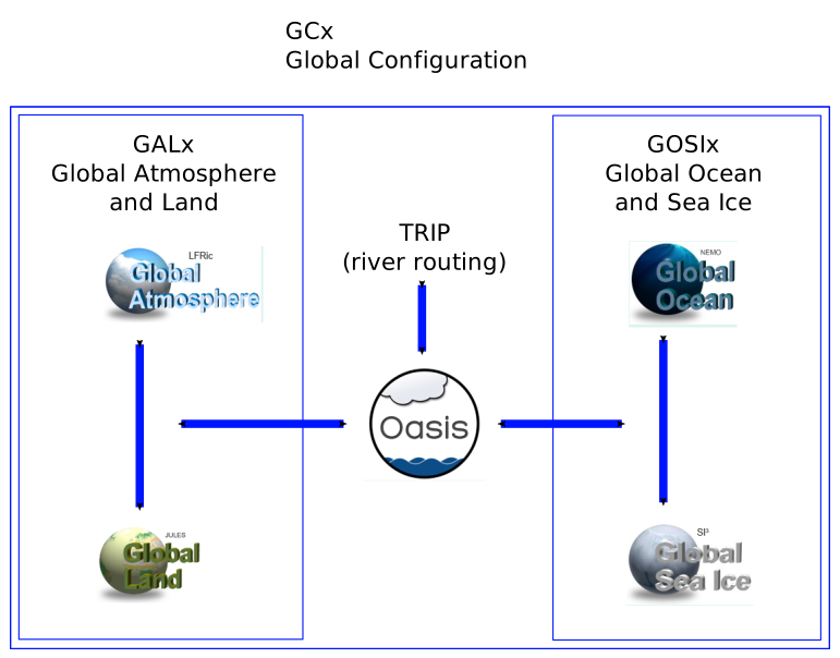
Fig. 21 Components coupling in a GC-LFRic configuration#
Within each of these combined systems, information is exchanged at every model timestep. This frequent exchange reflects the strong physical coupling between the relevant processes, such as energy, moisture, and momentum fluxes. As a result, the components must run within a single executable. This form of coupling is referred to as intra-model coupling.
The GAL and GOSI models are then further coupled to form the GC configuration.
Regional (Limited Area) Modelling#
Limited Area Models (LAMs), or regional models, simulate a restricted geographical domain at higher spatial resolution. They are designed to provide more detailed and locally relevant forecasts and projections for a specific region.
Why Regional Modelling?#
One of the primary scientific motivations for regional modelling is the challenge of representing deep convection. In global models, the horizontal grid spacing is often tens of kilometres. However, individual convective clouds are only a few kilometres wide. Because they are smaller than the grid spacing, they cannot be directly simulated. Instead, their effects are represented using a convection parameterisation scheme, which remains a significant source of uncertainty.
By contrast, regional models can operate at kilometre-scale resolution, allowing deep convection to be more explicitly represented within the model dynamics (although it is still not fully resolved). At these convection-permitting resolutions, the convection parameterisation scheme is typically switched off. This has been repeatedly shown to improve the simulation of the diurnal cycle of convection, the intensity of tropical cyclones, and the structure and intensity of convective systems such as open-cell convection.
In addition to improving the representation of convection, regional modelling is also motivated by the need for more detailed and locally relevant information. As a result, regional models are widely used for:
High-resolution NWP
Regional climate studies
Impact assessments (e.g. evaluating effects on flooding, agriculture, energy, and infrastructure)
They also allow for a much more realistic representation of surface features, including high-resolution orography. Accurately resolving valleys, hills, and mountains is critical for forecasting near-surface variables such as temperature, wind, and fog.
Key Characteristics of Regional Models#
Regional atmosphere–land systems have a number of distinguishing characteristics compared to global coupled models. In particular, they:
Use the same atmosphere and land components as global models
Operate over a limited spatial domain
Require lateral boundary conditions, provided by a global driving model, or a coarser-resolution regional model
Run at higher horizontal resolution than global models, typically from ~4 km down to <100 m
Can include additional scientific complexity at a fraction of the cost of running equivalent resolution globally
Higher resolution also introduces important numerical considerations:
Shorter timesteps are required for numerical stability
This can lead to faster responses in instantaneous variables
As a result, outputs may require different interpretation compared to global model counterparts
Using a high-resolution regional model driven by lateral boundary conditions from a larger-scale model allows finer-scale processes to be resolved while maintaining consistency with the large-scale weather patterns.
Fun fact!
LFRic, pronounced “elfrick”, was named after Lewis Fry Richardson, a pioneering British mathematician who made significant contributions to the field of numerical weather prediction. His methods laid the groundwork for modern weather forecasting, and the name LFRic pays homage to his legacy in atmospheric science.