The unstructured world#
Unstructured meshes and the UGRID format represent the future of scientific data delivery. As computational models evolve, especially in the realm of climate and weather modelling, transitioning to these new formats will be crucial for effective data handling.
Important
The unstructured world section will explore how unstructured data is transforming workflows, why it is important, and how scientists can adapt their practices to support these advancements.
Unstructured meshes offer greater flexibility and precision compared to structured grids, making them essential for data evaluation and verification. The section will explore the challenges and benefits of unstructured data and the technical details of using the UGRID format.
Features of unstructured meshes in the LFRic Atmosphere model#
Thanks to its use of an unstructured mesh, LFRic atmosphere offers greater flexibility, scalability, and precision. Some benefits of using an unstructured mesh instead of a structured grid are:
Improved Resolution: Unstructured meshes provide more accurate representations of complex shapes and regions, allowing for higher-resolution simulations.
Flexibility: Unstructured meshes can easily adapt to different features like coastlines and mountains without changing the grid.
Efficiency: LFRic improves computational efficiency by optimizing resource use and supporting advanced parallelization.
Scalability: Unstructured meshes enable higher-order methods, making it easier to scale models for larger, more detailed simulations.
To fully benefit from these features, working with unstructured data and understanding the UGRID format, which efficiently handles this type of data, is essential. Fig. 9 shows examples of unstructured meshes.
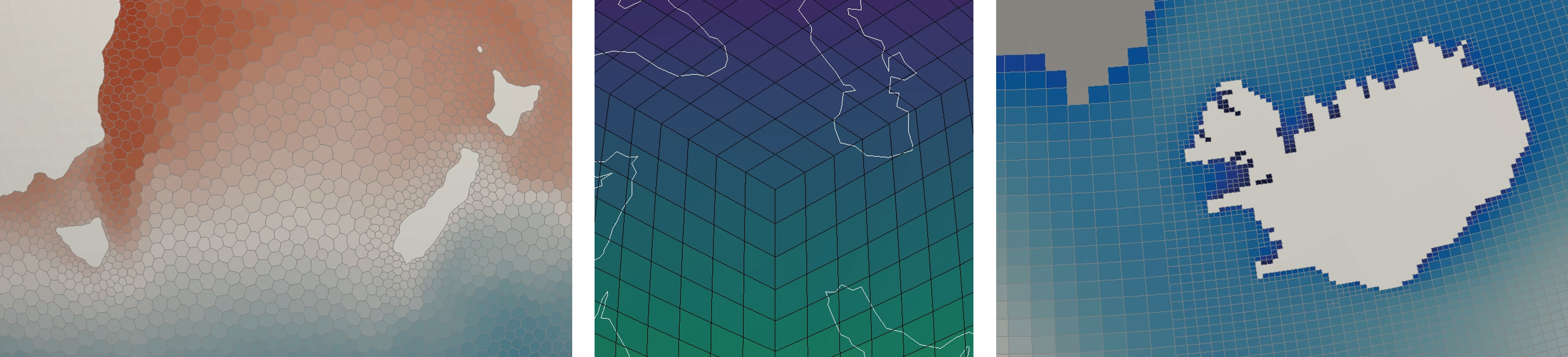
Fig. 9 Examples of unstructured meshes used in scientific computing.#
UGRID description of unstructured data#
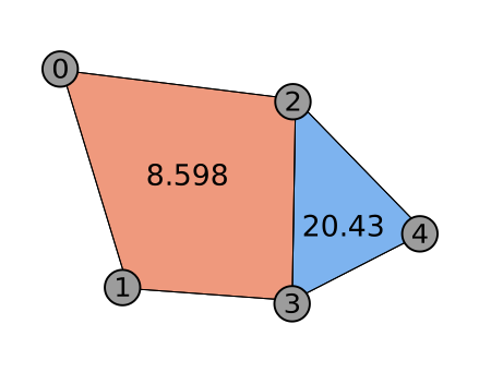
Fig. 10 UGRID mesh elements showing data stored on faces#
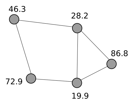
Fig. 11 UGRID mesh elements showing data stored on nodes#
The UGRID format is more flexible than structured grids because the nodes, edges, and faces do not need to align with predefined grid lines, such as latitude or longitude. Consequently, the spatial position of an element is independent of its position along the grid dimensions, offering a much more adaptable system. Additionally, the UGRID format allows for mixing faces of different geometries, including 3-sided, 4-sided, 5-sided, and even n-sided faces. This further increases the flexibility of the mesh, allowing for complex geometries that structured grids cannot accommodate.
In the context of our LFRic atmosphere unstructured mesh, all model data will be placed either on faces or edges, never on the nodes. For instance, data such as fluxes and vectors typically resides on edges, while other physical quantities are placed on faces.
Furthermore, each vertical layer shares the same horizontal coordinates, simplifying data handling across layers.
This unstructured mesh approach, which permits mixing different face geometries and the freedom to attach data to various mesh elements, demonstrates a level of flexibility that is difficult to achieve with structured grids.
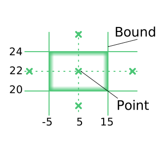
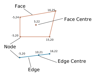
To highlight the differences between unstructured and structured grids, let’s consider how cells are described. In the structured grid approach, cells are described using points and bounds, defining the area between upper and lower bounds.
In the unstructured mesh approach, cells are described using a variety of elements, including faces, face centers, nodes, node centers, and edges. Each element is independently described, providing more flexibility and precision.
One key distinction is that in the mesh approach, each element is assigned its own description. In contrast, in structured grids, a single bound is used to describe the entire cell, which can lead to greater efficiency when describing certain elements (e.g., a line). However, this efficiency comes at the cost of flexibility, as the structured approach is less adaptable to complex geometries.
The two figures below contrast the structures of grids and meshes.
Managing unstructured data#
When working with unstructured data, the amount of data to handle increases significantly. For example, imagine 5 million cells are arranged on a flat layer. In the case of the Unified Model (UM) on the left, 13,400 data points (points and bounds) are needed to describe the entire space. However, in the unstructured case, because everything is described individually, around 40 million data points are required to represent the same space.
Structured grid (UM 2560 × 1920) |
Unstructured mesh (LFRic C905) |
|
|---|---|---|
Data points |
4,900,000 |
4,900,000 |
Geospatial Data |
Points: 4,480
Bounds: 8,960
|
Nodes: 9,800,000
Face-node connectivity: 19,700,000
Face centre: 9,800,000
|
Geospatial total |
13,400 |
39,300,000 |
Flexibility vs. data volume#
To put this into perspective, imagine data is described by a newspaper. In the structured grid approach, it’s like reading a pamphlet—simple and compact. In the unstructured case, however, it’s like reading an entire novel. This illustrates an important concept:
Important
While unstructured data offers greater flexibility, it also comes with a higher data cost.
UGRID can support both 2D and 3D meshes. In the GungHo formulation, cells are 3D, and it’s even possible to represent LFRic data on a 3D UGRID mesh using irregular cubes. For example, fluxes could be represented on all six faces of a cube—four horizontal directions plus upward and downward directions. However, to minimize the amount of coordinate data and reduce processing time, we currently focus on 2D meshes for diagnostic data output, especially for typical use cases.
Complexity of operations#
Another consideration when working with unstructured data is the increased complexity of operations. In a structured grid, extracting data from a specific region is relatively simple. For example, in Fig. 14, to extract data from rows 3 to 4 and columns 3 to 5, the array can easily be sliced to extract that data.
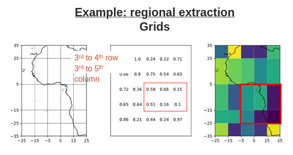
Fig. 14 Regional data extraction in a structured grid by slicing the array.#
Extracting data in unstructured meshes#
In unstructured meshes, the situation is more complex. Mesh data is one-dimensional, and there are no fixed latitude or longitude dimensions. Instead, the coordinates map to the mesh dimension. If you want to extract data from a specific region, such as a red box, the indices can be anywhere, making the operation less straightforward and requiring more computation.
Let’s consider an example. To find the location of a specific element, such as a face, you need to examine its connectivity and perform an indexing operation to fetch the relevant data. This process has to be repeated for all 5 million faces in the mesh. The operation involves determining which faces are within the specified region and which are not. This is a computationally intensive task, requiring specialized libraries and powerful computing resources.
When dealing with Limited Area Models (LAMs), we focus on a smaller section of the LFRic cube-sphere. While the LFRic LAM grids may appear similar to a structured lat-lon grid on the surface (using rotated poles and grid boxes arranged into rows and columns), LFRic will output UGRID data. Therefore, the UGRID tools and operations are also applicable to LFRic LAMs.
Cubed sphere mesh#
LFRic Atmosphere uses a cubed sphere mesh. Meshes are named after the number of cells along one edge of the cube. Fig. 15 shows a C16 mesh, which represents the Earth’s surface by 6 x 16 x 16 = 1536 cells (“squares”) in each horizontal layer. Most cell corners have four neighbour cells but at the corners of the cube only three cells meet.
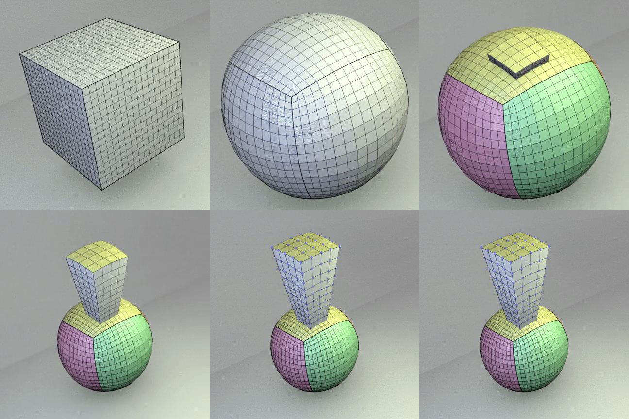
Fig. 15 Visualisation of a C16 mesh and how the mesh on a cube is projected to a sphere.#
The projection used to map squares on a cube surface to a sphere causes mesh sizes to have different lengths in km. Representative length scales for mesh resolutions are given in the table below.
LFRic Mesh |
≈ dx [km] |
|---|---|
C48 |
192.1 |
C128 |
72.0 |
C448 |
20.6 |
C896 |
10.3 |
C1808 |
5.1 |
C9216 |
1.0 |
Tools for unstructured data#
As described in the previous sections, LFRic is using an unstructured cubed-sphere mesh in the UGRID format. Understanding how to effectively work with this data requires the use of specialized tools.
Topic
In this section, attention will be given to: the tooling available for handling UGRID data and how these tools fit into the broader ecosystem.
A suite of common tooling was developed within the Scientific Python ecosystem, which provides a foundation for managing and analysing complex scientific data. This toolkit includes a variety of libraries and resources designed to assist in the manipulation of unstructured data formats, such as UGRID.
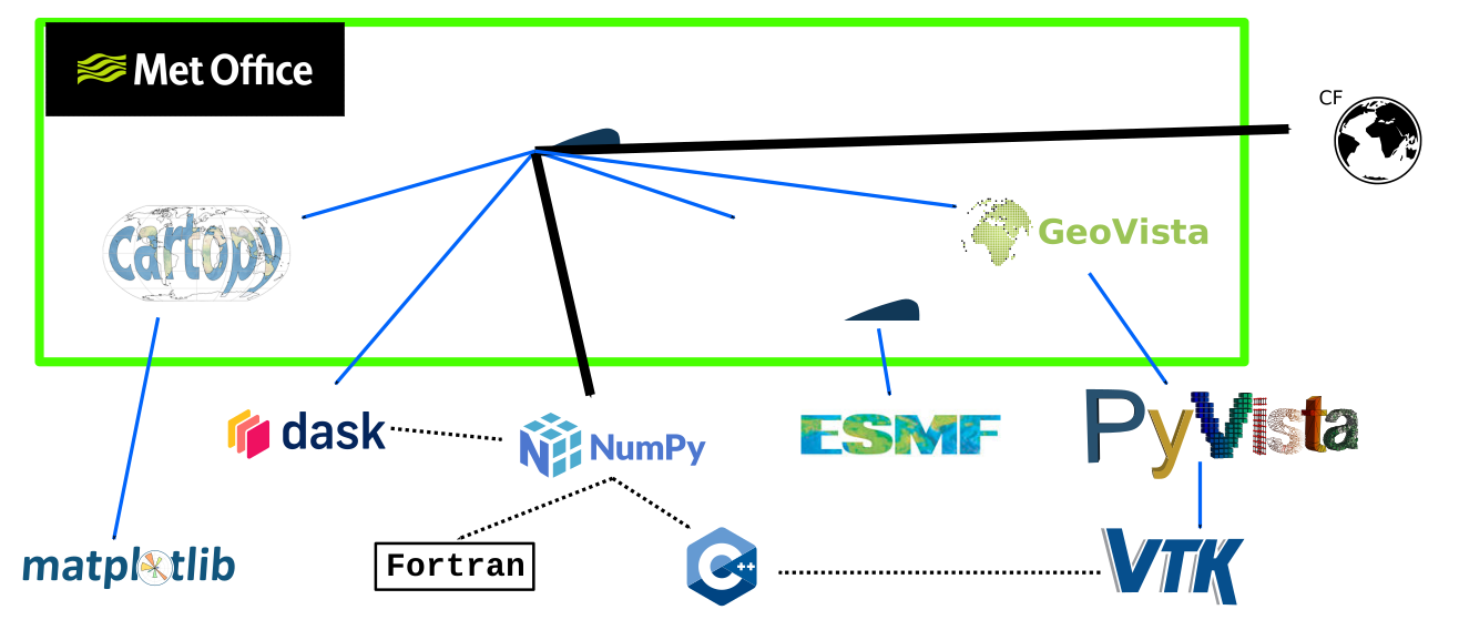
Fig. 16 The Scientific Python Ecosystem and unstructured data tools#
The main resources for the tools and standards shown in Fig. 16 are:
Iris: Iris documentation, Iris on GitHub
CF conventions: CF conventions project page
NumPy: NumPy documentation, NumPy on GitHub
Dask: Dask documentation, Dask on GitHub
Matplotlib: Matplotlib documentation, Matplotlib on GitHub
Cartopy: Cartopy documentation, Cartopy on GitHub
ESMF and iris-esmf-regrid: ESMF project page, ESMF on GitHub, iris-esmf-regrid documentation, iris-esmf-regrid on GitHub
PyVista: PyVista documentation, PyVista on GitHub
GeoVista: GeoVista documentation, GeoVista on GitHub
Despite the use of compiled languages such as Fortran and C++ in parts of the scientific Python stack, Python serves as the interface for data interaction with these tools during user workflows.
A widely used tool for handling scientific data is Iris. Iris is a powerful library that facilitates the analysis of meteorological and climate data, and it is specifically designed to work with both structured and unstructured grids. It offers a range of functions that simplify the manipulation and visualisation of data, making it a key component in many data processing workflows.
In this section, a brief overview of the basics of Iris will be provided, including its core features and functionalities.
Iris - basics and scope#
Iris is a Python-based ecosystem and package used for the manipulation of LFRic data during post-processing. It is open-source and has been included in other tools, such as ESMValTool and MetPlus, which are based on it. Iris offers a unified view of data as cubes and supports metadata-aware processing. It provides analysis capabilities in mathematics, statistics, large data handling, and regridding. For visualisation, Iris relies on Matplotlib and Cartopy.
The core of Iris is built around CF and NumPy. CF (Climate and Forecast) conventions allow Iris to work with the encoding of climate and forecast data stored in netCDF files. NumPy provides efficient array operations implemented in compiled code and linked numerical libraries, avoiding the performance limits of pure Python loops.
NumPy facilitates the mathematical operations required for large datasets. Operations involving substantial numerical processing are offloaded to efficient compiled implementations, while Python remains the user-facing interface.
Regridding unstructured data#
In the unstructured mesh context, ESMF (Earth System Modelling Framework) is utilised for regridding tasks. Regridding allows for comparison between datasets defined on different meshes, enabling analysis that requires data on specific local representations, such as OSGB (Ordnance Survey National Grid) in Britain, or requires computations suited to structured grids, like zonal means.
The regridding process in the unstructured world follows two primary steps: preparation and execution. During the preparation phase, the source and target grids are compared, and weights are calculated using ESMF. The preparation step is computationally intensive, particularly with unstructured grids. In the execution phase, the calculated weights are applied to the data, and a new cube is constructed. This phase typically involves Python libraries such as DASK and SciPy.
Different types of regridders are available depending on the source and target grid types. These include Mesh-to-Grid, Grid-to-Mesh, and Area-Weighted Regridders.
Each regridder offers various features, including the ability to read and write cubes, perform area-weighted regridding, and preserve metadata during operations. Additionally, the capability to load and save regridders is supported.
Masked data during regridding
Some datasets contain masked data: values that should not be used in analysis. During regridding, the source data mask is carried across to the target grid. If masked source data covers more than the configured threshold for a target cell, that target cell is masked too. Otherwise, the target cell remains unmasked.
Key features of regridding include:
flexibility in selecting regridders,
the ability to preserve metadata, and
efficient handling of masked data.
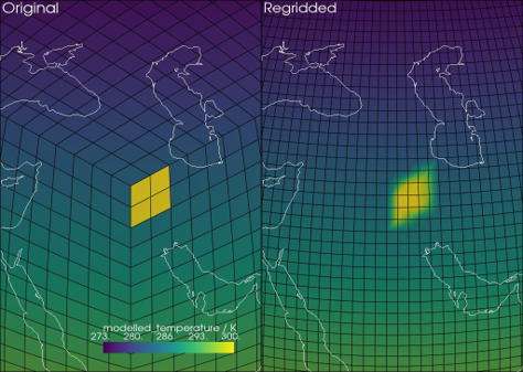
Fig. 17 Regridding data from an unstructured mesh to a structured grid#
The regridding tools discussed above are documented by the ESMF user guide, ESMF source repository, and iris-esmf-regrid documentation.
Visualising unstructured data#
Structured-grid workflows commonly use Matplotlib for 2D plotting, with Cartopy adding map projections and other cartographic features. Those tools remain useful for many latitude-longitude datasets, but they do not scale well to high-resolution unstructured meshes.
The unstructured workflow therefore uses tools built around 3D mesh rendering. PyVista provides Python access to the Visualization Toolkit (VTK), a C++ library for 3D visualisation and mesh processing. VTK can use GPU-accelerated rendering, which is important for datasets with many mesh faces. GeoVista adds geospatial and cartographic helpers on top of PyVista, performing a role similar to Cartopy for map-aware visualisation.
ParaView is another tool in this ecosystem. It is a parallel visualisation application for large scientific datasets.
See the subsections below for detailed package summaries and links.
PyVista - basics and scope#
PyVista is the main Python interface used here for rendering LFRic unstructured meshes. It gives Scientific Python users a NumPy-friendly API for 3D geometry, so they can build visualisation workflows without writing C++ code.
For the workflows covered in this training, PyVista supports:
interactive rendering in Jupyter notebooks;
batch (off-screen) rendering for automated workflows; and
mesh filters such as slicing, contouring, and interpolation, which support both visualisation and computational geometry tasks.
The performance advantage over Matplotlib becomes significant at LFRic resolutions. For example:
Mesh |
PyVista time |
Matplotlib time |
|---|---|---|
C48 (approximately 13,000 faces) |
approximately 370 ms |
approximately 14 s |
C1048 |
under 4 s |
approximately 2 hours |
GeoVista - basics and scope#
GeoVista is an open-source Python package that adds cartographic capabilities to PyVista, fulfilling a role analogous to Cartopy in the structured-grid world. It helps transform geospatial data into PyVista meshes for interactive 3D rendering, including unstructured meshes such as cubed-sphere LFRic output.
GeoVista supports longitude-latitude data, unstructured meshes, coastline overlays, texture mapping, and regional extraction (e.g. cropping a cubed-sphere dataset to a specific geographic region). Its current projection support is more limited than Cartopy’s but includes common geographic rendering workflows and selected projected outputs. Because GeoVista uses the same rendering stack as PyVista, it can display the high face-count datasets associated with operational LFRic resolutions.