Install and run the CSET cylc workflow

This tutorial provides a step by step guide of how to run CSET via its included cylc workflow comparing data from multiple forecasts, resulting in a website of plots to navigate.

Prerequisites

The CSET workflow uses cylc 8, so you must ensure that is the version of cylc configured for use on your system. You can check whether cylc is available with the following command:

Caution

The example shell snippets in this documentation use bash, and may not work with other shells. In particular there are known issues activating conda environments with ksh.

# Check version starts in 8.
cylc --version

Install the command line

The CSET cylc workflow is included with the CSET command line program. Therefore, the first thing you will need to do is to install the CSET command line.

The recommended way to install CSET is via conda. It is packaged on conda-forge in the cset package. The following command will install CSET into its own conda environment, which is recommended to avoid possible package conflicts.

conda create --name=cset --channel=conda-forge cset

To use CSET, you need to activate the conda environment with the conda activate command.

conda activate cset

Note

You will need to rerun the conda activate cset command whenever you use a new terminal.

Once that is completed, CSET should be ready to use. This can be verified by running a simple command.

cset --version

This command should output the installed version of CSET. This will look something like CSET vX.Y.Z.

Install the workflow

With the newly created conda environment activated, run the cset extract-workflow command to unpack the workflow from inside the CSET package into a directory of your choosing. A sensible choice is ~/cylc-src, which is the default location where cylc will search for workflows.

# Create the cylc-src directory if it doesn't exist.
mkdir -p ~/cylc-src
# Extract the workflow from CSET into the chosen directory.
cset extract-workflow ~/cylc-src
# Change into the freshly unpacked workflow directory.
cd ~/cylc-src/cset-workflow-vX.Y.Z

Your directory should look like this:

$ ls
app  conda-environment  includes                     lib   opt        rose-suite.conf.example
bin  flow.cylc          install_restricted_files.sh  meta  README.md  site

If you are at a site with specific CSET integration, such as the Met Office or Momentum Partnership, you will want to install the site specific configuration files that specify where cylc will run the tasks. This is done by running the install_restricted_files.sh script. For other users, you can skip this step and use the localhost site instead.

./install_restricted_files.sh

You have now installed the CSET workflow and are ready to use it.

Download sample data

We will now download some sample data containing screen level air temperature and air temperature on pressure levels for two sample forecasts, for two different models to help us explore some of the functionality of CSET. The tutorial data consists of 4 files to download:

File	Size
MODELA_20230117T0000Z.nc	~20 MiB
MODELA_20230118T0000Z.nc	~20 MiB
MODELB_20230117T0000Z.nc	~90 MiB
MODELB_20230118T0000Z.nc	~90 MiB

Download these files and save them somewhere persistent, such as your home directory or a SCRATCH disk. You can download via your browser or directly copy these links and use wget to retrieve on the command line.

Workflow configuration

After downloading the CSET release and the data to evaluate, we next set up the required CSET configuration. Take a copy of the rose-suite.conf.example configuration file to create a copy rose-suite.conf in the same directory. This can be edited from inside the cset-workflow-vX.Y.Z directory using the rose edit command.

# Copy the example file to create a fresh rose-suite.conf.
cp rose-suite.conf.example rose-suite.conf
# Edit the configuration with the rose edit GUI.
rose edit

You should now have a graphical program with which you can navigate the various configuration settings that CSET provides. Detailed help for each setting can be accessed by clicking the setting’s name.

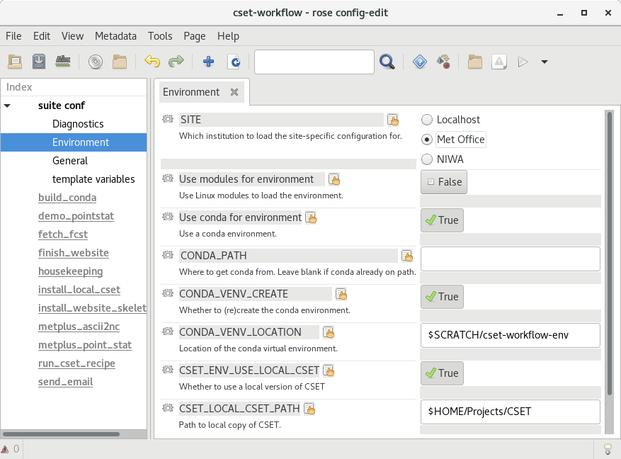
General setup options

Expand the top level suite conf heading of the navigation tree to the left hand side of the GUI, go to the General setup options panel, and set the following settings:

• Select the Site or set Localhost if not listed.

• Adjust the Web directory to point to a directory that is served by your webserver. Often this is a directory like ~/public_html.

• (Optionally) set the Website Address to the URL where your web directory is served. This is the address your will use to display your results in a webbrowser.

Hint

rose edit is somewhat unreliable. Frequently click the save button to avoid losing entered information when navigating to a new page.

Cycling and Model options

Next select the Cycling and Model options panel in the left hand navigation tree, and set the following:

• Leave the Cycling mode selected as Case Study.

• Add the two required Case study dates to evaluate. The example data for this tutorial has two forecasts initialised on "20230117T0000Z" and "20230118T0000Z".

• Set the Analysis length as PT48H to indicate a 48-hour forecast length.

• Set the Number of models to 2, as we want to assess two different models.

• Keep Cutout Subarea set to False.

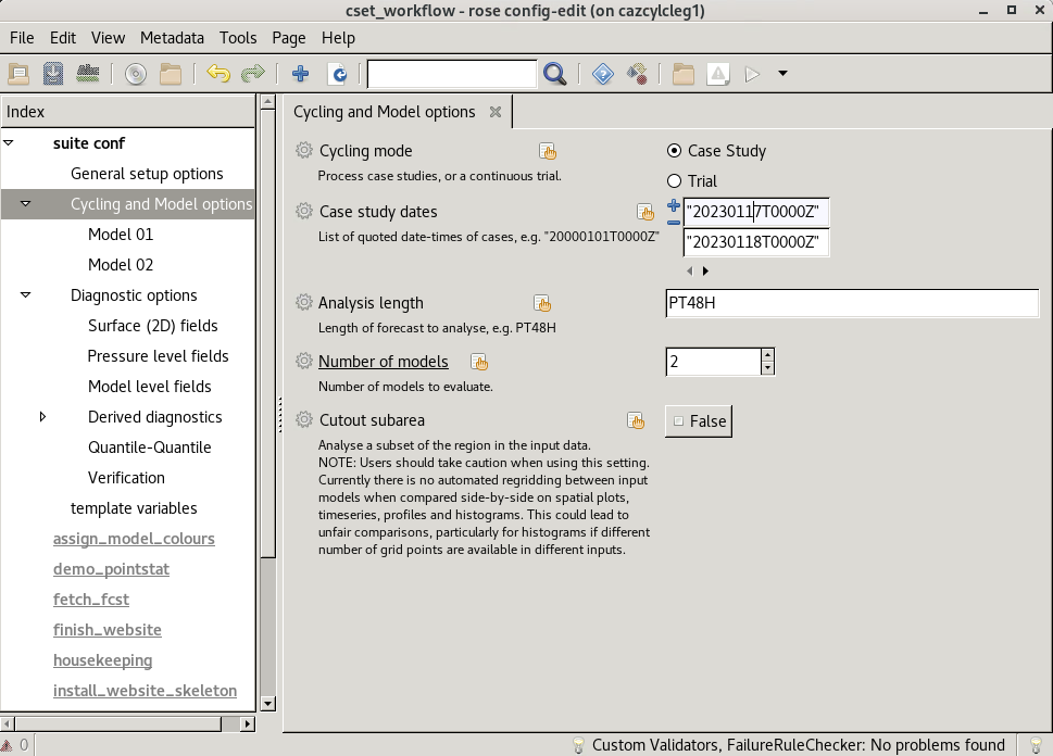
Setting the number of models activates new Model 01, Model 02, … panels in the navigation tree in which to specify model-relevant settings. You may need to further expand the navigation tree to see them.

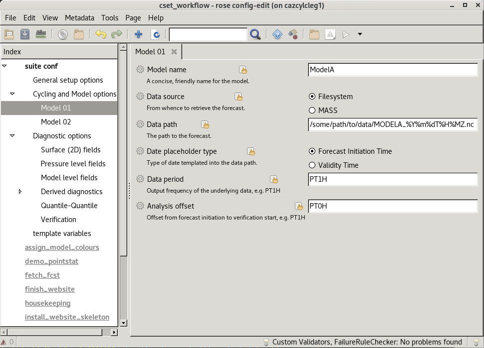
Navigate to each Model panel by expanding the Cycling and Model options menu in turn to set model-specific settings:

• Add a readable Model name which will be associated with the data in CSET outputs.

• Select Filesystem as the Data source to indicate that the test data is on a locally mounted disk.

• Enter the path to data, including wildcards and formatting to specify filename structure. This should follow the format /some/path/to/data/MODELA_%Y%m%dT%H%MZ.nc, providing a unique path to the data files. The % components in the file path will evaluate the filename based on the case study date.

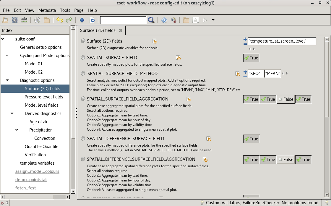
Diagnostic options

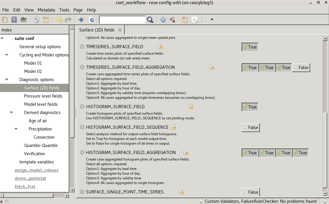
Next expand the Diagnostic options panel and open the Surface (2D) fields panel.

This panel provides option for processing and visualising variables that are only defined on a single diagnostic level such as, but not exclusively, surface fields. Set the following settings:

• Click the + option to add a variable name to Surface (2D) fields and add "temperature_at_screen_level". This setting lists all 2D variables of interest from the input data that CSET will process.

• Set SPATIAL_SURFACE_FIELD to True to enable plotting of spatial maps.

• Set SPATIAL_SURFACE_FIELD_METHOD to "SEQ" and "MEAN". These are the aggregation methods used by the spatial plotting. The SEQ method will produce a series of output maps for every time through the forecast (typically hourly), while the MEAN method will produce spatial plots meaned over forecast period. Multiple methods can be specified in this list to generate all within the same CSET workflow run.

• Set the first, second, and fourth SPATIAL_SURFACE_FIELD_AGGREGATION options. This sets the methods for generating aggregated summary maps across case studies computed as a function of lead time, hour of day, validity time, or to generate a single map summarising all input data across all forecast periods.

• Set SPATIAL_DIFFERENCE_SURFACE_FIELD to True to enable plotting of difference map plots comparing the two models.

• Set the first, second, and fourth SPATIAL_DIFFERENCE_SURFACE_FIELD_AGGREGATION options, enabling aggregated differences across multiple cases.

• Set TIMESERIES_SURFACE_FIELD to True to enable domain mean (or sub-area) time series plots.

• Set the first, second, and fourth TIMESERIES_SURFACE_FIELD_AGGREGATION options, enabling time series across multiple cases.

• Set HISTOGRAM_SURFACE_FIELD to enable plotting of histograms.

• Set the first, second, and fourth HISTOGRAM_SURFACE_FIELD_AGGREGATION options to control plotting of aggregated outputs across forecasts.

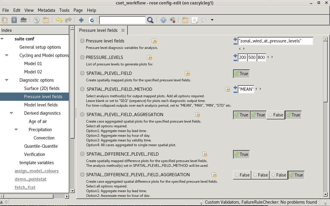
Next, to add a 3D variable of interest, open the Pressure level fields panel. Standard options for variables defined on multiple levels (e.g. pressure levels or vertical model levels) are similar, and editable on the relevant sub-panel selected from the left hand navigation tree. Set the following:

• Add "zonal_wind_at_pressure_levels" to the list of Pressure level fields.

• Add 200, 500, and 850 to the list of PRESSURE_LEVELS, the pressure levels on which to generate outputs.

• Set SPATIAL_PLEVEL_FIELD to True to enable spatial plots on each selected pressure level.

• Set SPATIAL_DIFFERENCE_PLEVEL_FIELD to True to enable plotting of spatial differences.

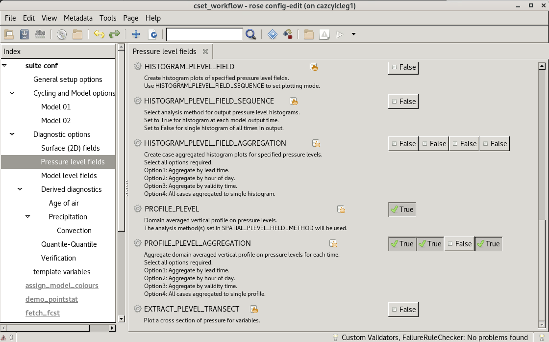
• Set PROFILE_PLEVEL to enable vertical profile plots of the domain mean. This will only generate profiles from the PRESSURE_LEVELS selected (i.e. data at 200 hPa, 500 hPa and 850 hPa in this example), so ensure the number of requested levels is sufficiently high to generate the required vertical resolution outputs.

• Set the first, second, and fourth PROFILE_PLEVEL_AGGREGATION options.

Ensure you save the configuration before closing rose edit. Once saved, you can validate your configuration with cylc validate to check for missed settings or unexpected values.

# Perform some quick checks to make sure the metadata is valid.
cylc validate .

Run the workflow

After configuration via the rose GUI, the CSET workflow is ready to run.

To run the workflow, use cylc vip within the cset-workflow-vX.Y.Z directory. You can view the job’s progress in the browser with the cylc GUI, accessible with the command cylc gui, or in the terminal with cylc tui.

# Run workflow from within the cset-workflow-vX.Y.Z directory.
cylc vip .
# Monitor the workflow's progress.
cylc gui

Other commands to control the workflow are described in the cylc running workflows documentation.

Once CSET has finished running you will receive an email containing a link to the output page.

View CSET outputs

Once completed, the CSET workflow will send an email to confirm successful completion and link to outputs at the web address specified in the GUI.

Outputs are stored in the web directory, located in ~/cylc-run/cset-workflow-vX.Y.Z/runN/share/web (or an equivalent cylc-run path if running the CSET workflow with a specified run name).

Warning

If you cylc clean the workflow, this will delete the plot directory. To keep the plots independently of the workflow directory, move the web directory to a required alternative location and update the symlink to the web directory back to the Web directory location from which CSET outputs are displayed.

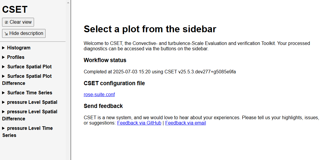
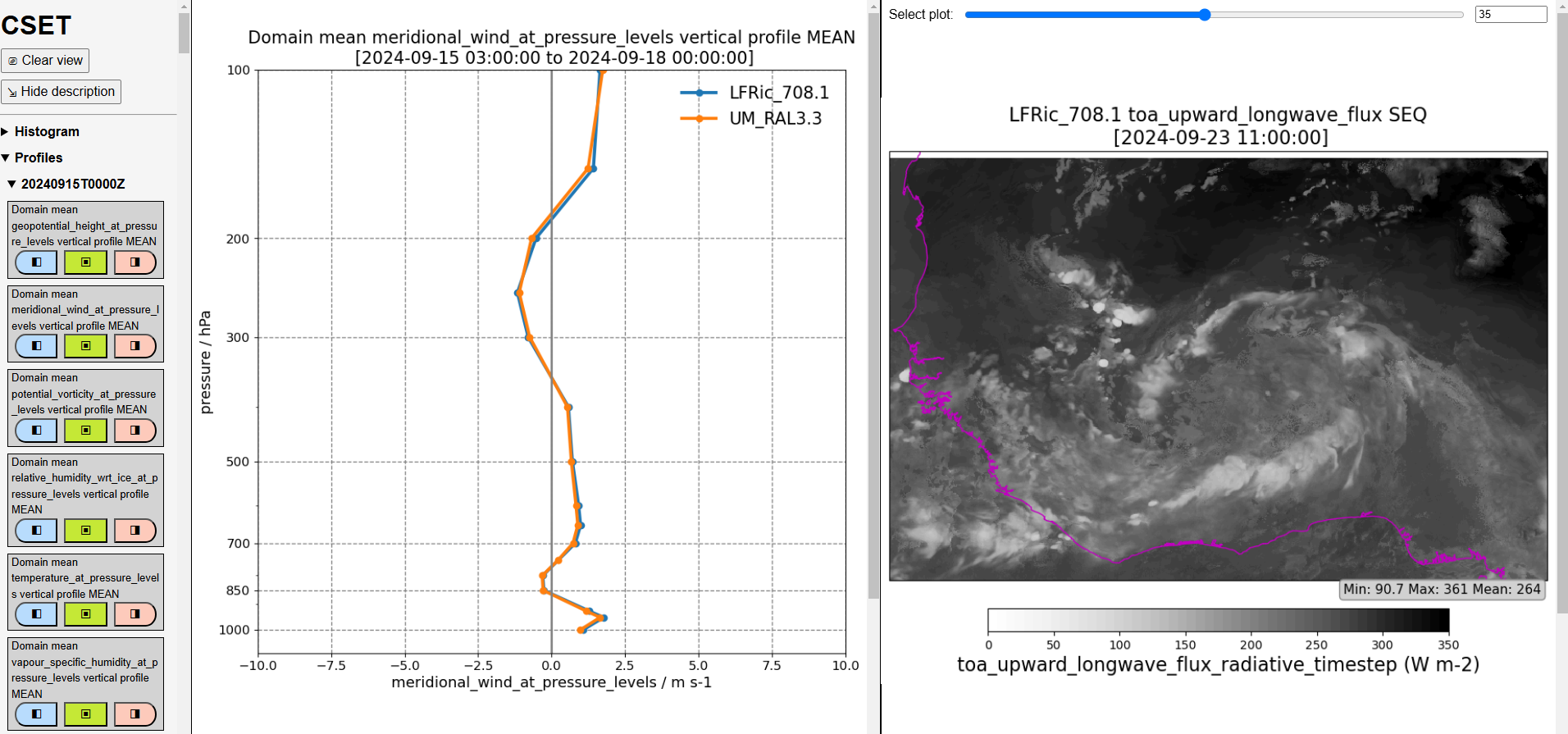
CSET web outputs can be navigated using the sidebar organised by type of plot, and by forecast date and aggregations. Plots can be displayed in either left-hand, central, or right-hand web views.

You have now run the CSET workflow! Take some time to explore the output webpage. You can find further information on configuring the workflow in Configure the workflow.