

Attention
This documentation has been transferred directly from the UM to LFRic; (UMDP 024: The Parametrization of Boundary Layer Processes). It is still a work in progress. There are still UM-specific references and terminology that are yet to be updated.
The Parametrization of Boundary Layer Processes#
- Author:
Lock, J. Edwards and I. Boutle
Introduction and code versions#
This is the documentation for the “boundary layer” parametrization of vertical turbulent transports of heat, moisture and horizontal momentum. It includes surface exchange but not the parametrization of the surface itself. This is covered within the surface (JULES) documentation. Although commonly referred to as the “boundary layer” parametrization, it includes a free-tropospheric component. Turbulent fluxes are calculated up to “BL_LEVELS” which is currently set so that the entire troposphere is included.
Generally speaking, only version 9C of the boundary layer parametrization will be documented here as it is now the only supported version. However, the documentation still makes occasional references to previous versions of the scheme (8A, 9B) as it is useful to retain the history of how we have got to where we are. Version 9 interfaces to the JULES surface code, which is now the only supported surface code within the UM.
Several options for higher order closures are available in the 1A
version of the UM boundary layer scheme and these are documented
separately in :umdp:025.
Model variables and turbulence closure#
Given source terms, \({\mathcal{S}}\) say, from processes other than boundary layer turbulence, Reynolds’ averaging gives the following equation for conserved scalar variables, \(\chi\), and the two horizontal components of momentum, \({\mathbf{u}}\) on a sphere gives:
where \(\overline{w'\chi'}\) and \({\bf \tau}\) are the vertical turbulent fluxes to be parametrized, \(r\) is the height from the centre of the planet and \(\rho\) is density. The scalar variables treated by (207), which are approximately conserved under moist adiabatic ascent, are:
where \(T\) is temperature, \(q_v\) is specific humidity, \(q_{\ell}\) and \(q_f\) the specific liquid and frozen water contents respectively, and \(L_s=L+L_f\) is the latent heat of sublimation. Note that \(\theta_{\ell}\) is based on ‘liquid/frozen water static energy’ (\(= c_p T + g z - L q_{\ell}- L_s q_f\)) rather than potential temperature, \(\theta\). Note also that the option to use mixing ratios in the boundary layer code instead of specific quantities is also available and the details of the necessary changes are documented in appendix Appendix: changing between specific humidities and mixing ratios. Ultimately turbulent motions are dissipated as heat and so the source term \({\mathcal{S}}\) in (207) can include an approximation for that frictional heating, as described in appendix Appendix: including the heating from turbulence dissipation. Finally, the ice cloud contributions in (209) and (210) can optionally be ignored (l_noice_in_turb), which will be more appropriate if the time scales for ice melting or sublimation are longer than those of the turbulence (and so may be more appropriate if the ice itself is not being mixed by parametrized turbulence). In this instance the saturation humidity will be calculated with respect to liquid water at all temperatures and, for consistency, only liquid cloud fractions with be considered.
An additional variable used for diagnostic purposes is
where \(c_v=(1/\epsilon) -1\) and \(\epsilon\) is the ratio of the molecular weights of water vapour and dry air (i.e., \(\epsilon = M_v/M_a \approx 0.62198\)). Thus \(\theta_{v\ell}\) is a conserved variable that is equal to virtual potential temperature (\(\theta_v\)) in cloud-free air and so is used as a simplified measure of buoyancy.
A ‘first-order’ closure is used to parametrize the turbulent fluxes, although non-local terms are also included. Under the 9C scheme, an alternative methodology is optionally available, see section The revised scalar flux-gradient formulation. The standard closures are:
Separate eddy-diffusivities are calculated for momentum, \(K_m\), and for scalar variables, \(K_h\). The second term on the right hand side represents a non-local flux in unstable boundary layers. Currently it is only applied for transport arising from surface-driven turbulence (\(K_h^{\mathrm{surf}}\)) and is non-zero only for \(\chi=\theta_{\ell}\), as described in section Gradient adjustment.
Thus, the parametrization reduces to determining \(K_h\), \(K_m\) and \(\gamma_{\chi}\) and \({\bf \tau}^{nl}\). Two methods are used to determine \(K_h\) and \(K_m\) and how they are combined for (212) and (213) is described in section Shear-driven mixing and interaction between the local and non-local schemes. The first method is a local Richardson number (\(Ri\)) based scheme. It is calculated for all regimes (but will be responsible for all mixing in stable conditions), over all levels up to the specified BL_LEVELS and is described in section The local scheme. The second method is a non-locally specified profile scheme. This is exclusively for unstable boundary layers, is calculated up to level NL_BL_LEVELS (typically around 6km AMSL) and is described in more detail in section The non-local scheme. In this regime, mixing is assumed to occur in (or lead rapidly to the formation of) well-mixed layers (in which conserved variables are approximately uniform with height) that are capped by an inversion. Mixing is assumed to be driven either from the surface in a ‘surface mixed layer’ (SML, by a positive surface buoyancy flux and by surface stresses) or by cloud-top buoyancy sources (radiative and evaporative cooling, see appendix Appendix: Definitions of the velocity scales). As described in section The non-local scheme, separate \(K\)-profiles are used for these two turbulence sources. If the cloud-top sources generate mixing throughout the SML the layer is said to be ‘coupled’ but if the \(K\)-profile representing surface-driven mixing does not extend up to cloud-top, the layer is referred to as being ‘decoupled’. As decoupled layers are restricted to being buoyancy driven and typically below 6km, they are referred to as decoupled stratocumulus (DSC) layers. The calculation of \(\gamma_{\chi}\) is described in section Gradient adjustment and, finally, fluxes across the top of both SML and DSC layers (the entrainment fluxes) are specified explicitly through a separate entrainment parametrization, as described in section Entrainment fluxes.
The strategy used to determine precisely where and when the resulting eddy-diffusivities should be applied is described in section Diagnosis of boundary layer depth and type. The buoyancy parameters, finite difference and other notation used here are defined in appendices Appendix: Derivation and definitions of the buoyancy parameters and Appendix: Notation. Further papers describing this scheme and its performance are Lock et al. (2000) (noting the corrigendum in Lock et al. (2001)), Martin et al. (2000), Lock (2001), Bush et al. (1999) and Brown et al. (2008).
Diagnosis of boundary layer depth and type#
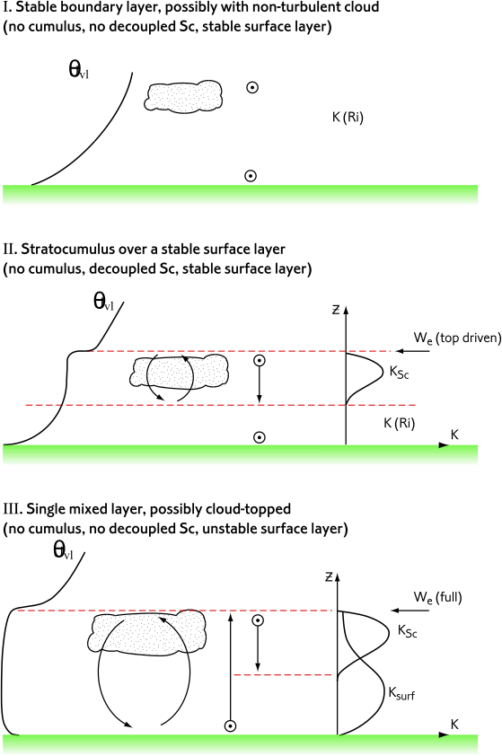
The non-locally specified \(K\)-profiles require the height of the base and top of the layer to be diagnosed (see section The non-local scheme). Furthermore, as stated in section Model variables and turbulence closure, the mixing generated by the non-local \(K\) profiles is assumed to occur in (or lead rapidly to the formation of) well-mixed layers capped by an inversion. Thus, the accurate diagnosis of their vertical extent is crucial. How to make this diagnosis is dependent on the boundary layer mixing regime which has been categorised into 7 distinct ‘boundary layer types’:
Type I: Stable boundary layer (with or without cloud) – turbulent diffusivities are calculated by the ‘local’ scheme (section The local scheme)
Type II: Boundary layer with stratocumulus over a stable near-surface layer – as Type I but with a turbulently mixed cloud layer driven from its top (a DSC layer, diagnosis described in section Diagnosis of the vertical extent of the K-profiles)
Type III: Well mixed boundary layer – the classic single mixed layer which may be cloud-topped or clear but is predominantly buoyancy-driven (c.f. a possible type VII below) – diagnosis described in section The diagnostic parcel ascent and cumulus diagnosis)
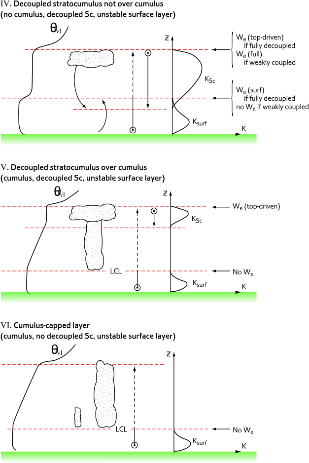
Type IV: Unstable boundary layer with a DSC layer not over cumulus (see section Diagnosis of the vertical extent of the K-profiles) – the surface-based and cloud-top-driven non-local \(K\) profiles may or may not overlap and cloud-top entrainment can still include the surface forcing (see section Entrainment fluxes)
Type V: Boundary layer with a DSC layer over cumulus – the cumulus (treated by the model’s mass-flux convection scheme) provides coupling with the SML (cumulus diagnosis described in section The diagnostic parcel ascent and cumulus diagnosis)
Type VI: Cumulus-capped boundary layer – no turbulent diffusivities are allowed [1] at or above the LCL as the mass-flux convection scheme operates here (cumulus diagnosis described in section The diagnostic parcel ascent and cumulus diagnosis)
Type VII: Shear-dominated unstable layer – potentially wind-shear might allow deeper turbulent mixing in unstable boundary layers than is apparent purely from the thermodynamic profiles (sufficient even to inhibit the formation of cumulus); the possibilities are discussed in section Shear-driven mixing and interaction between the local and non-local schemes.
Types I to VI are shown schematically in Fig. 4.

Fig. 4 Schematic representation of boundary layer types I to VI. The top of the upward arrows indicate the height \(z_{\mathrm{par}}\) while the top of their solid line portions indicate \(z_{\mathrm{h}}\).#
|
|
The diagnostic parcel ascent and cumulus diagnosis#
Summary: the depth of the non-local \(K\)-profiles for surface-driven turbulence (with NTML grid-levels in the mixed layer and top at height \(z_{\mathrm{h}}\) , as required for (234)) is determined from:
a diagnostic moist parcel ascent; top at grid-level NTPAR, height \(z_{\mathrm{par}}\) \(=z_{\mathrm{ \mathrm{NTPAR}}+\frac{1}{2}}\). Typically this is an adiabatic parcel but entraining options are available.
a diagnosis of cumulus-capped layers (if cumulus-capped then NTML and \(z_{\mathrm{h}}\) are set to the LCL [2], if not then to the parcel top)
Note that this process is only performed for unstable boundary layers (defined by a positive surface buoyancy flux, i.e., \(\overline{w'b}_S>0\)).
Step 1: the method assumes that the height to which turbulent mixing driven by surface processes can extend in unstable boundary layers (and therefore the vertical extent of the \(K\) profile for surface-driven turbulence) can be determined solely from the properties of the thermodynamic profiles. In more detail, the first step in calculating \(z_{\mathrm{h}}\) is to lift a parcel, with properties from the first grid-level (\(k=k_s\)) above the top of the surface layer, upwards allowing for latent heat release. The top of the surface layer is taken to be at the lower of \(z=0.1\)\(z_{\mathrm{h}}\) (this is then consistent with the \(K\)-profiles, see section Surface-driven turbulence; \(z_{\mathrm{h}}\) is taken from the previous timestep) and the grid-level above which \(\theta_{v\ell}\) starts to increase with height. The ascent is stopped at the grid-level NTPAR (height \(z_{\mathrm{par}}\) \(=z_{\mathrm{ \mathrm{NTPAR}}+\frac{1}{2}}\)) above which the parcel becomes more negatively buoyant than a given threshold, \(\theta_v'\). Note that the parcel properties themselves are not perturbed in order to preserve the height of the mixed-layer’s lifting condensation level (LCL). The calculation of the parcel’s buoyancy excess is described in section Calculation of parcel buoyancy excess. Currently,
where \(A_{plume}=0.2\), \(B_{plume}=3.26\), \(G_{max}=10^{-3}\)Km\(^{-1}\), \(\sigma_{Tv1} = 1.93\, \overline{w'\theta_v'}_S/w_m\) and \(w_m^3=u_*^3+0.25\,z_{\mathrm{h}}\overline{w'b}_S\). Following Holtslag and Boville (1993), \(\theta_v'\) is related to the magnitude of the gradient adjustment, \(\gamma_{\theta_{\ell}}\) (see section Gradient adjustment). Thus, \(B_{plume}=A_{ga}\), although somewhat arbitrary limits have been placed on the magnitude of \(\theta_v'\) for numerical security (the upper limit being consistent with that applied to \(\gamma_{\theta_{\ell}}\) in (239) ). Within limits, then, \(\theta_v'\) represents a typical buoyancy excess of boundary layer plumes.
The pressure at the LCL, \(P_{LCL}=P_{k_s} (T_{LCL}/T_{k_s})^{(1/\kappa)}\), where \(\kappa=R/c_p\). The temperature at the LCL, \(T_{LCL}\), is calculated using approximations in Bolton (1980) as
where the vapour pressure of air in grid-level \(k_s\), \(e_{k_s} = q_{k_s} P_{k_s}/(100 \, \epsilon)\). The full-level below that containing the LCL is labelled NLCL and \(z_{\mathrm{lcl}}\) \(=z_{\mathrm{ \mathrm{NLCL}}+\frac{1}{2}}\). If the parcel rises above the top of the LCL transition zone (defined as 1.1\(z_{\mathrm{lcl}}\) , its ascent can also be stopped at the grid-level at which it has maximum buoyancy excess over the environment. This is identified as the grid-level above which
where currently the tolerance for identifying inversions by this method, \(\Gamma_{\mathrm{inv}}=1.1\). This use of the height of maximum excess (if lower than that given by the straight buoyancy threshold, \(\theta_v'\)) is typically of little consequence in stratocumulus regions (which tend to be well-mixed beneath large inversions), but can be necessary in order to identify the capping inversion in cumulus cases (e.g. in the trade wind regions).
Step 2: having established \(z_{\mathrm{par}}\) , a crucial additional test is to determine whether this layer is well-mixed (i.e., stratocumulus-capped) or cumulus-capped. The parcel ascent can rise to cloud-top in both cases but cumulus cloud layers are observed not to be as well-mixed as stratocumulus layers. Recall that application of the \(K\) profiles is expected to form or maintain well-mixed layers and so their current formulation is inappropriate for cumulus cloud layers. Specifically, a logical flag (CUMULUS) is set to true if
where the cloud-layer gradient, \(\Delta_{\mathrm{cld}}\), is taken between both NTPAR and NTPAR-1 (to allow for the possibility that a Sc layer has just deepened by a grid-level) and NLCL and the sub-cloud layer gradient, \(\Delta_{\mathrm{sub}}\), between grid-levels NLCL and \(k_s\). Currently the threshold factor, \(C_t = 1.1\). If cumulus is diagnosed, the top of the surface-based mixed layer (\(z_{\mathrm{h}}\) ) is set to \(z_{\mathrm{lcl}}\) (rather than to \(z_{\mathrm{par}}\) , as illustrated in Fig. 4 for types V and VI). There is then an option to diagnose the thickness of the LCL transition zone, see section Diagnosis of the LCL transition zone thickness. Otherwise, the boundary layer surface-driven mixing is capped at \(z_{\mathrm{lcl}}\) so that mixing into the cumulus cloud layer is only carried out by the model’s mass-flux convection scheme and not by the eddy viscosity based boundary layer scheme. Note that basing the CUMULUS diagnosis on cloud and sub-cloud layer gradients limits the model only to being able to resolve cumulus with cloud and sub-cloud layers at least 2 grid-levels (and optionally 400m) thick. Otherwise the layer is considered well-mixed to \(z_{\mathrm{par}}\) with an option to include a representation of fluxes into the capping inversion (see section Diagnosis of inversion thickness).
If the parcel ascent fails to find an inversion below 3km (or BL_LEVELS) but the LCL is below BL_LEVELS, then the layer is assumed to be cumulus-capped. If the LCL is above BL_LEVELS, then again cumulus is diagnosed with NTML\(=\mathrm{min}[\)NLCL, BL_LEVELS\(-1]\), in the hope that the mass-flux convection scheme (in its moist or dry mode) will transport the surface fluxes higher! Clearly this restriction on the boundary layer scheme is not desirable and so a value of BL_LEVELS above the tropopause is recommended.
Note that if cumulus is not diagnosed then a further, subgrid estimation of the height of the capping inversion is attempted for \(z_{\mathrm{h}}\) (as described in section Diagnosis of a sub-grid inversion).
Calculation of parcel buoyancy excess#
As described in appendix Appendix: Derivation and definitions of the buoyancy parameters, virtual temperature, \(T_v = T(1 + c_v q_v - q_{\ell}- q_f)\), is used as the measure of buoyancy. The condensed water in the parcel at a grid-level \(k\) (\(q_{\ell f}^p\), the superscript \(^p\) indicating parcel properties) is estimated using a Taylor expansion of \(q_s\) about the environment at that grid-level (\(q_s^p \approx {q_s}_k + \alpha_L (T^p-T_k)\)). Assuming that \(q_{\ell f}^p=q_t^p - q_s^p\) gives
where the buoyancy parameters \(a_L\) and \(\alpha_L\) are defined in appendix Appendix: Derivation and definitions of the buoyancy parameters. Recall that the parcel has \(q_t\) and \(\theta_{\ell}\) taken from grid-level \(k_s\) which are conserved during its ascent. Note that (215) will not give condensation until the parcel becomes saturated. In the environment the cloud scheme will allow some condensation (and therefore warming and stabilisation of the environment profile) to take place before the grid-level becomes saturated in the mean. To allow for this in the parcel (without applying the cloud scheme), (215) is also calculated at each grid-level but using the environment grid-box mean \(q_t\) and \(\theta_{\ell}\) to give \(q_{\ell f}^e\). The difference in the environment’s condensed water as determined by the UM cloud scheme (i.e., \(q_{\ell}+q_f\)) and by (215) (i.e., \(q_{\ell f}^e\)) is then added to \(q^p_{lf}\).
Given \(q_{\ell f}^p\), (209) implies \(T^p = \theta_{\ell}^p - (g z_k/c_p) + (L q_{\ell f}^p/c_p)\) (using \(L_s\) if \(T_k\) is below the melting point) and (210) implies \(q_v^p = q_t^p - q_{\ell f}^p\) and thus \(T_v^p\) can be calculated. Recall that the diagnosis of the parcel’s maximum buoyancy excess over the environment (described in section The diagnostic parcel ascent and cumulus diagnosis) required \(\theta_v\). This is approximated as \(\theta_v = T_v + (g z_k/c_p)\).
Diagnosis of the vertical extent of the K-profiles#
The diagnosis of mixed layers with turbulence driven from cloud-top has been separated in to three stages. These are:
diagnose the existence of a decoupled stratocumulus (DSC) layer with approximately uniform \(\theta_{v\ell}\) (label the top grid-level in the mixed-layer NTDSC and diagnose the subgrid height of its capping inversion, \(z_{\mathrm{h}}^{\mathrm{Sc}}\) , see section Diagnosis of a sub-grid inversion)
diagnose an approximate depth of the DSC layer, \(z_{\mathrm{ml}}\), in order to be able to calculate the representative turbulent velocity scales (see appendix Appendix: Definitions of the velocity scales).
calculate the depth of the \(K\) profiles (see section The non-local scheme) in both SML and DSC layers using constraints on the TKE budget of the layer. This includes the diagnosis of recoupling of DSC layers and decoupling of SMLs
Step 1: the diagnosis of DSC layers depends on whether cumulus convection has been diagnosed. If a cumulus-capped layer under an inversion within BL_LEVELS has been diagnosed, grid-levels NTPAR and NTPAR+1 are tested to see if they contain significant layer cloud (\(C_F>\) SC_CFTOL). This threshold for identifying potentially turbulently-mixed cloud layers is currently SC_CFTOL\(=0.1\). If there is significant cloud, NTDSC is set to NTPAR.
Alternatively, if a well-mixed surface-driven boundary layer was diagnosed, then from grid-level NTML\(+2\) upwards, a cloud-top grid-level (\(k_{ct}\)) is sought such that \({C_F}_{k_{ct}}>\) SC_CFTOL and \({C_F}_{k_{ct}+1}<\) SC_CFTOL. If \(\Delta_{k_{ct}} \theta_{v\ell}/ \Delta_{k_{ct}} z < 10^{-3}\)Km\(^{-1}\) (i.e., \(\theta_{v\ell}\) is approximately well-mixed over at least two grid-levels), then NTDSC is set to \(k_{ct}\). If grid-levels \(k_{ct}\) and \(k_{ct}-1\) are not well-mixed, grid-levels \(k_{ct}-1\) and \(k_{ct}-2\) are tested using the same criterion. If they are not well-mixed either, the cloud-layer is ignored for the purposes of turbulent mixing. If grid-levels \(k_{ct}-1\) and \(k_{ct}-2\) are identified as well-mixed a further test is applied to determine whether the \(\theta_v\) (rather than \(\theta_{v\ell}\)) gradient across grid-levels \(k_{ct}\) and \(k_{ct}-1\) is greater than adiabatic (i.e., whether grid-levels \(k_{ct}\) and \(k_{ct}-1\) actually form part of an inversion – note that by ignoring the \(q_{\ell}\) contribution to buoyancy, \(\theta_{v\ell}\) is not a good variable to use to measure the strength of cloud-capping inversions). To do this, the \(\theta_v\) gradient between grid-levels \(k_{ct}\) and \(k_{ct}-1\) is compared with that for a parcel lifted adiabatically from grid-level \(k_{ct}-1\), in exactly the same way as for the SML parcel ascent (see section Calculation of parcel buoyancy excess). If \(d\theta_v/dz|_{\mathrm{env}} > \Gamma_{\mathrm{inv}} d\theta_v/dz|_{\mathrm{par}}\) between grid-levels \(k_{ct}\) and \(k_{ct}-1\) then NTDSC is set to \(k_{ct}-1\); if not then NTDSC is set to \(k_{ct}\) (recall that grid-levels \(k_{ct}-1\) and \(k_{ct}-2\) have already been identified as well-mixed).
Step 2 is to diagnose an approximate depth of the DSC layer, \(z_{\mathrm{ml}}\). The bottom grid-level of the mixed-layer (NBDSC) is diagnosed as the lowest grid-level, descending from NTDSC, where \({\theta_{v\ell}}_{\mathrm{ \mathrm{NTDSC}}} + \theta_{v\ell}'\) is less than \(\theta_{v\ell}\) of the environment. The parcel perturbation is given by
where \(\Delta_F\) (Kms\(^{-1}\)) is the magnitude of the cloud-top radiative divergence (see appendix Appendix: Definitions of the velocity scales), \(\tau_{rc}\) is a timescale for the exposure of boundary layer eddies to the cloud-top radiative cooling (taken to be 200s) and \(z_{rc}\) is a depth-scale for the radiatively cooled layer (taken to be 50m). These values of \(\tau_{rc}\) and \(z_{rc}\) are only estimates (and will in reality vary from one cloud to another) but they are consistent with, for example, the observations of Nicholls and Turton (1986). If the parcel failed to fall (i.e., NBDSC equals NTDSC) in a DSC layer not overlying cumulus, then the layer is assumed not to be well-mixed. At the top of a cumulus layer, the DSC layer is given a minimum depth of \(\Delta_{\mathrm{ \mathrm{NTDSC}}+\frac{1}{2}} z\). Otherwise, the layer depth, \(z_{\mathrm{ml}}\), is measured from the top of layer NTDSC to the base of layer NBDSC.
Step 3: the step 2 calculation of \(z_{\mathrm{ml}}\) is used to calculate the representative velocity scales for the DSC layer but its calculation is only crude. Here, the vertical extent of the \(K\)-profiles is determined more accurately by ensuring that the magnitude of the integrated buoyancy consumption of TKE within the mixed layer is less than or equal to a fraction, \(D_t\), of the buoyancy production, following Turton and Nicholls (1987).
Following appendix Appendix: Derivation and definitions of the buoyancy parameters the grid-box mean buoyancy flux can be written as:
As standard, the fluxes in (217) are then expanded using the first-order closure in (212) as:
where \(\widetilde{\Delta_k \theta_{\ell}} = \Delta_k \theta_{\ell}- \gamma_{\theta_{\ell}} \Delta_k z\) in order to include the non-local (or gradient adjustment) term. If the alternative flux-gradient option is used, see section The revised scalar flux-gradient formulation, then additional terms are needed.
Large-eddy simulations have demonstrated that the crucial region in determining when decoupling of stratocumulus will occur (i.e., when the \(K\) profiles no longer span the entire layer from cloud-top to the surface) is in a thin layer of unsaturated air just below cloud-base, where \(\overline{w'b}\) first becomes negative. Thus, in the above calculation, it is crucial both to have an accurate measure of cloud-base height (which will have to be subgrid) and to include successfully this thin unsaturated layer in the buoyancy consumption integral. Thus, the \(\overline{w'b}\) integration is performed over the cloud and sub-cloud layers separately and the cloud-fraction is taken to be uniform within the cloud layer (and zero below cloud-base). The height of cloud-base is given by (466).
An iterative method is then used to find the vertical extent of mixing (within certain bounds, as described below) such that the magnitude of buoyancy consumption of TKE within the mixed layer equals a fraction, \(D_t\), of the buoyancy production, i.e.,
Note that, for simplicity, the \({\mathcal{E}}_h\) factors are not included in \(K_h^{\mathrm{surf}}\) or \(K_h^{\mathrm{Sc}}\) when calculating (218) under the assumption that they will be small. This process is applied to all unstable mixed layers. For stratocumulus layers, observations and LES suggest a value of \(D_t=0.1\). A separate value of \(D_t\) can be used for the sub-cloud layer in cumulus capped boundary layers if this method is used to determine the LCL transition zone thickness, see section Diagnosis of the LCL transition zone thickness. For cloud-free mixed layers, \(D_t=1\) is used, purely to keep negative buoyancy fluxes down to a reasonably realistic level (for example, if the parcel top diagnostic returned too high a boundary layer depth).
The first step is to test for whether a well-mixed layer is possible (either decoupling what has so far been diagnosed as a well-mixed layer or, if one exists, recoupling a decoupled stratocumulus layer), i.e., to test whether (219) is satisfied with both \(K_h^{\mathrm{surf}}\) and \(K_h^{\mathrm{Sc}}\) extending from the surface to the cloud-top. If recoupling is possible then the various flags identifying the DSC layer are reset (this includes setting the cumulus diagnosis to false), any surface-driven entrainment originally applied at \(z_{\mathrm{h}}\) is added to the entrainment at \(z_{\mathrm{h}}^{\mathrm{Sc}}\) (after rescaling for the inversion strength at \(z_{\mathrm{h}}^{\mathrm{Sc}}\) ) and \(z_{\mathrm{b}}\) is set to 0.1\(z_{\mathrm{h}}\) (for the reason discussed above). If decoupling is diagnosed, \(z_{\mathrm{h}}^{\mathrm{Sc}}\) is set to the original \(z_{\mathrm{h}}\) (inversion height), although the entrainment across this inversion is not recalculated (and so keeps any surface-driven component – the COUPLED flag is therefore set to true, see section Entrainment fluxes).
If a decoupled layer is diagnosed, then an iteration is performed to find the highest \(z_{\mathrm{h}}\) (so top of the \(K_h^{\mathrm{surf}}\) profile) that still satisfies (219), but with \(K_h^{\mathrm{Sc}}=0\) in (218). The iteration proceeds with \(z_{\mathrm{h}}\) stepping from its lowest permissible height to its highest (currently 3 steps are used). If at any stage (219) is violated, then the step below (therefore containing the height that would give equality in (219)) is divided by 4 and 3 of those steps are taken downwards. If (219) is met the step above is again reduced by a factor of 4 and 3 steps taken upwards. A total of 3 sweeps are possible, each with a smaller step so that \(z_{\mathrm{h}}\) approaches the height that gives equality in (219). The accuracy with which this is achieved will be the difference in the maximum and minimum permissible heights of \(z_{\mathrm{h}}\) divided by \(2\times4\times4 = 32\), which will typically be less than 30m. The top grid-level of the SML, NTML, is defined as the highest grid-level such that \(K_h^{\mathrm{Sc}}\) is non-zero at the half-level above.
The above process is then repeated to find the appropriate \(z_{\mathrm{b}}\) for \(K_h^{\mathrm{Sc}}\), i.e., for the base of top-driven mixing. Some constraints are placed on \(z_{\mathrm{b}}\) , namely that it should never go below \(0.1\)\(z_{\mathrm{h}}\) (to avoid affecting the continuity of the \(K\) profiles at the top of the surface layer, see (235)). If cumulus convection has been diagnosed then \(z_{\mathrm{b}}\) is not allowed to go below \(z_{\mathrm{ \mathrm{NTML}}+\frac{1}{2}}\) (unless the layer is diagnosed to recouple completely). Finally, \(z_{\mathrm{b}}\) must always be at or below \(z_{\mathrm{ \mathrm{NTDSC}}-1}\), so that mixing in decoupled layers is always resolved, and at least \(\Delta z_{rad}\) (the cloud-top radiative cooling depth defined in section Integration of overline{w’b} close to the inversion) below the t inversion. The base grid-level of the DSC layer, NBDSC, is defined (analogously to NTDSC) as the lowest grid-level such that \(K_h^{\mathrm{Sc}}\) is non-zero at the half-level below.
A possible extension to this diagnosis would be to include the shear contribution to the TKE budget in (219) and so allow shear-driven mixing to help maintain well-mixed layers.
Surface layer \(\overline{w'b}\) integration#
In the surface layer, below \(z_i/10\), the \(K\) profiles have a different functional form from the rest of the mixed layer. Rather than include this additional complexity in the \(\overline{w'b}\) integration, the surface layer is treated separately. In place of the finite-difference form of \(\overline{w'b}\), see (217) and (218) above, \(\overline{w'b}\) is assumed to be linear between \(\overline{w'b}_S\) at the surface and zero at a level which must be estimated. The surface layer integration is then from the surface up to \(z_{{\mathrm{K}_{SURF}}}\), where \(\theta\)-level K_SURF is the first above \(z_i/10\). The level where \(\overline{w'b}\) is zero is found by linear interpolation across the grid-levels where the diagnosed cloud-free buoyancy flux would become negative. This is where \(\beta_T \widetilde{\Delta_k \theta_{\ell}} + \beta_q \Delta_k q_t\) becomes positive and so where the cloud-free part of \(\overline{w'b}\) (i.e., that part below cloud-base which is important for decoupling) becomes negative.
Integration of \(\overline{w'b}\) close to the inversion#
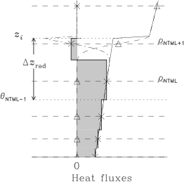
Because of the large gradients often seen in fluxes close to the inversion (in particular, in the LW radiative flux), simple finite difference flux calculations, (218), can be significantly inaccurate in this region. An example is shown in Fig. 5. Calculating \(\overline{w'\theta_{\ell}'}_{\mathrm{ \mathrm{NTML}}+\frac{1}{2}}\) from (218) gives a negative value, largely because \(\Delta_{\mathrm{ \mathrm{NTML}}+1} \theta_{\ell}\) is positive and so the local flux is large and negative. In reality, \(\overline{w'\theta_{\ell}'}\) becomes positive only a short distance below cloud-top such that the integral here will tend also to be positive.
The solution adopted is to integrate \(\overline{w'b}\) analytically across the region just below the inversion, labelled \(\Delta z_{rad}\) in Fig, 5. Since \(\Delta_{\mathrm{ \mathrm{NTML}}} \theta_{\ell}\) can also be significantly positive (when the grid-level inversion is rising or falling, for example), the base of this region is taken to be the lower of the first \(\theta\)-level below \(z_h-100\) m (a physically reasonable depth over which cloud-top radiative cooling might be expected to occur) and \(z_{\mathrm{ \mathrm{NTML}}-1}\).
Fig. 5 Subgrid (lines) and model (symbols) fluxes of \(\theta_{\ell}\): turbulent flux (dash-dotted, crosses), radiative flux (dashed, triangles) and total flux (solid). The shaded area illustrates the integrated turbulent flux that would be obtained were (218) used.#
|
Then,
For the radiative flux, it could be assumed that the subgrid flux distribution is exponentially dependent on the grid-level LWP, for example. This would give:
However, off-line tests indicated this could give a strong and spurious sensitivity to \(F^{rad}|_{z_h-\Delta z_{rad}}\). Furthermore, for most realistic scenarios, the logarithmic factor in (221) tends to be close to 3. Consequently, we approximate \(I^{rad} = \Delta z_{rad} ( F^{rad}|_{z_h}-F^{rad}|_{z_h-\Delta z_{rad}} ) /3\). In addition, \(F^{rad}|_{z_h}-F^{rad}|_{z_h-\Delta z_{rad}}\) is approximated as \(\Delta F\), the radiative flux change across cloud-top used in the calculation of \(V_{\mathrm{Sc}}\) (468). The precipitation flux is assumed to vary linearly across this region, as does the total flux, and so its contribution to \(I^{Tot}\) cancels with \(I^{ppn}\) in (220). Finally, for simplicity, the total flux is taken to be constant and equal to the inversion value, such that \(I^{Tot} = \Delta z_{rad} F^{Tot}|_{z_h}\). With these approximations, (220) becomes
For the integral of \(\overline{w'q_t'}\) across this cloud-top region, \(\overline{w'q_t'}\) is also taken to be constant so that:
The integrated buoyancy flux is then found from (217) using the mixed layer cloud fraction and buoyancy coefficients evaluated at the grid-level above \(z_h -\Delta z_{rad}\).
Diagnosis of inversion thickness#
Terminating the diagnostic parcel ascent at its level of neutral buoyancy ignores any overshooting through the parcel’s own inertia as it enters the inversion region. This overshooting region effectively defines the depth of the inversion over which the negative entrainment heat fluxes are seen. Typically this will be small relative to the model vertical grid but at higher vertical resolution or when a strongly surface-heated boundary layer is capped by weak stability inversions could be resolved. Following Beare (2008), a simple energetic argument gives a realistic prediction of the top of the inversion, \(z_{top}\), in LES from
where \(z_{nb}\) is the level of neutral buoyancy (found by linear interpolation between grid-levels), \(w_m\) is the boundary layer velocity scale defined in section Surface-driven turbulence and \(b\) is the parcel buoyancy. Note that the constant in (222) is the same as in Beare (2008) because \(6.3 = 2.5 * 4^{2/3}\) and \(w_m^3\) differs by a factor of 4. The buoyancy integration in (222), that is itself dependent on \(z_{top}\), is performed working upwards from \(z_{\mathrm{par}}\) assuming piece-wise linear variation of \(b\) between grid-levels. Note that the standard definition of the boundary layer top in the UM is the height of the first flux level below the level of neutral buoyancy, so \(z_{\mathrm{par}}\) \(=z_{\mathrm{ \mathrm{NTPAR}}+\frac{1}{2}}\). The inversion thickness is then defined as
Diagnosis of the LCL transition zone thickness#
As described in section The diagnostic parcel ascent and cumulus diagnosis, when cumulus convection has been diagnosed surface-driven mixing was originally capped at \(z_{\mathrm{lcl}}\) so that mixing into the cumulus cloud layer was only carried out by the model’s mass-flux convection scheme. This was seen to lead to errors in the mean profiles across the LCL, with superadiabats being the most extreme manifestation. Using the boundary layer parametrization to couple cloud and sub-cloud layers would have the numerical advantage of being implicit. There is also observational and LES evidence that appropriately-scaled buoyancy fluxes up to the LCL are indistinguishable from those in cloud-free convective boundary layers and so the non-local surface-driven mixed layer K-profiles remain accurate up to this level. To diagnose the depth to which these profiles should penetrate above the LCL, the algorithm given in section Diagnosis of the vertical extent of the K-profiles to diagnose the extent of the K-profiles in decoupled boundary layers can be used (using the switch kprof_cu). This ensures that the magnitude of the integrated buoyancy consumption of TKE within the mixed layer is less than or equal to a fraction, \(D_t\), of the buoyancy production. In cumulus layers, cloudy thermals will generate positive buoyancy fluxes (and are handled by the convection scheme) but it is assumed that there will also be cloud-free thermals within the grid box that may penetrate above the grid-box mean LCL (but are too dry to reach their own LCL). Thus their buoyancy flux is given by (217) with \(C_F=0\). Restricting the negative integral of this buoyancy flux then gives a new definition for \(z_{\mathrm{h}}\) that is then used in the calculation of the surface-driven K-profiles in section Surface-driven turbulence – the larger the value of \(D_t\), the higher \(z_{\mathrm{h}}\) will be. Typically \(D_t=0.1\) for decoupled stratocumulus layers while idealised clear-sky convective boundary layers (where the magnitude of the entrainment buoyancy flux is a fraction, \(A_1\), of the surface flux) would have \(D_t = A_1^2 \sim 0.05\). For GA7 \(D_t\) has been set to 0.05 for this cumulus transition zone calculation. Because the Gregory-Rowntree convection scheme triggers from the LCL, that is used as a minimum constraint on the boundary layer mixing depth (so that the massflux and turbulence schemes remain coupled). With other convection schemes this may not be appropriate and so this minimum constraint can be relaxed, which is achieved by setting it to half the height of the LCL (the factor of a half is arbitrary, with no sensitivity to this choice given that the diagnosis parcel reached the LCL, but ensures the iteration starts well below the LCL).
The local scheme#
A first order ‘mixing length’ closure is used:
where \({\mathcal{L}}_m\) and \({\mathcal{L}}_h\) are the neutral mixing lengths and \(S\) is the resolved vertical shear of the horizontal wind components, \(S = \left| \partial {\mathbf{u}}/\partial z \right|\). A representation of the wind shear, \(S_d\), generated by drainage flows in complex terrain can also be included, as described below. Near the surface simple finite difference calculations for the vertical gradients can become inaccurate because of the quasi-logarithmic profiles of variables [Ayra (1991)]. Currently this is ignored above grid-level 2 and the neutral mixing lengths are given by
where \(z_{0m}\) includes the orographic component. For the lowest interior grid-level (\(k=1\)) they are calculated, incorporating this log profile correction, as
If near-surface resolution is increased this logarithmic correction should be considered over more levels.
The asymptotic mixing lengths are given by
where \(\lambda_0\) is a minimum mixing length read in from the namelist and \(z_{\mathrm{loc}}\) is defined below. The orographic blending height, \(h_B\) (only used within the boundary layer, as defined below), is given by
where \(\sigma_h\) is the standard deviation of the height of the subgrid orography and \((z_{0m})_{\mathrm{veg}}\) is the vegetative part of the roughness length. The constants in (226) can be considered ‘tuned’ (see, in particular, the operational modifications described in appendix Appendix: Operational modifications).
The Richardson number, \(Ri\), that is used as a local measure of stability is given by
The measure of buoyancy used in \(Ri\) is
where \(\overline{\beta_T}\) and \(\overline{\beta_q}\) are the grid-box mean (i.e., cloud weighted) buoyancy coefficients, that can be defined in two different ways, see appendix Appendix: Derivation and definitions of the buoyancy parameters and section Finite difference calculations. Note that (228) reduces to a virtual temperature approximation of buoyancy in cloud-free air and that neutral buoyancy (in cloudy as well as cloud-free air) is implied by vertically uniform \(\theta_{\ell}\) and \(q_t\). This is then entirely consistent with the assumption that \(\theta_{\ell}\) and \(q_t\) are conserved variables within the boundary layer scheme.
As described in Lock (2012), the wind shear generated by drainage flows in complex terrain is thought to lead to additional vertical mixing. This wind shear can be approximated as
The representative slope of the local terrain, \(\alpha_d\), is given by
with \(l_h\) a specified horizontal scale for the terrain, currently taken to be 1500 m (empirically derived for Scottish orography in the UKV), and \(\sigma_h\) the standard deviation of the full subgrid orographic height. \(\sigma_h\) should also be taken as the average over the surrounding area of each grid box (typically 6 to 8 grid lengths), in order to be representative of the local area over which such flows will be underresolved. The above formula is used so that \(\alpha_d \sim \sigma_h/l_h\) for small \(\sigma_h\) but only tends to 0.2 for large values. To limit the vertical extent of \(S_d\) to be below approximately \(z=\sigma_h\), a height-dependent factor is included, \({\mathcal{Z}}_d = 0.5( 1 - {\mathrm{tanh}}\left[ 4 ((z/\sigma_h)-1) \right])\). The timescale, \(t_d\), takes a fixed value of 30 minutes, for simplicity.
Initially, the lowest half-level at which \(Ri>Ri_{crit}\) is taken to be a measure of the boundary layer top (\(z_{\mathrm{loc}}\) ) and the full-level below is designated NTLOC. In general \(Ri_{crit}=1\) but a value of 0.25 is recommended for use with the ‘SHARPEST’ stability functions, see below. If the boundary layer was diagnosed as cumulus-capped by the non-local scheme (see section Diagnosis of boundary layer depth and type) then \(z_{\mathrm{loc}}\) is lowered to \(z_{\mathrm{lcl}}\) (and \(K_h\) and \(K_m\) are set to zero from the base of grid-level NLCL upwards) so that transports into and within the cumulus cloud layer can be performed solely by the mass-flux convection scheme. Depending on the switch local_fa, above NTLOC turbulently-mixed layers (where \(Ri<Ri_{crit}\)) are identified and within each layer \(z_{\mathrm{loc}}\) in (226) is set to the layer thickness. Outside of these turbulent layers the mixing lengths are set to \(\lambda_0\).
For \(Ri < 0\), the standard UM stability functions are given by
with \(g_0=10\), \(D_m=g_0/4\) and \(D_h=g_0/25\). If the stability dependent Prandtl number option is chosen (see below) the neutral Prandtl number, \(Pr_N\), is set to \(0.7\); otherwise \(Pr_N=1\). Alternatives are those from the Met Office large-eddy model (LEM), Brown (1999) 2:
where \(Pr_N = 0.7\), and the constants \(b_{LEM}\) and \(c_{LEM}\) can take the values 40 and 16 respectively in the “standard” LEM model or both be 1.43 in the “conventional” model.
For stable conditions (\(Ri > 0\)), several forms for the stability functions are available. The ‘long-tailed’ functions are
Alternative functions, which decrease as \(1/Ri^2\) with increasing stability are, from Louis (1979):
and the family of “sharp” functions can be written in terms of a transitional Richardson number, \(Ri_{t}\), as:
where
For the ‘SHARPEST’ function of Derbyshire (1997), \(Ri_{t}=0.1\), while larger values give even sharper reduction of turbulence with increasing \(Ri\). An additional option, used operationally in some configurations (originally in the Mesoscale Model, hence called ‘MES tails’), is to blend linearly from Louis functions at the surface to SHARPEST by 200m.
A stability dependent Prandtl number (\(Pr=f_m/f_h\)) is generally used following Mailhot and Lock (2004) with:
The maximum permitted Prandtl number, \(Pr_{\mathrm{max}}\), is currently set to \(5\) for model stability reasons. The stability functions for \(Ri>0\) are then given by:
Note that writing the functions in this way ensures that \(f_m=1\) under neutral conditions and the effect of the variation in \(Pr\) is for \(f_m\) to decrease slower with increasing \(Ri\) than \(f_{\mathrm{stable}}\), which can be explained through increasing gravity-wave activity.
Finally, the LEM stable functions are also available which cut off all turbulence beyond a critical Richardson number, \(Ri_c=0.25\):
with \(g_{LEM}=1.2\).
Finite difference calculations#
The Charney-Phillips vertical grid staggering used in the UM stores the horizontal wind components (\(u\), \(v\)) on grid-levels, \(\rho\)-levels, that are staggered relative to scalar variables (such as \(\theta_{\ell}\) and \(q_t\)) and vertical velocity, \(w\). While much of the boundary layer scheme is grid-independent, this has serious implications for the calculation of \(Ri\). There are two obvious possibilities, to calculate \(Ri\) (and thence \(K(Ri)\)) on either \(\theta\)-levels or \(\rho\)-levels and then interpolate either \(K_h\) or \(K_m\) to be able to calculate the required fluxes. To do the former requires averaging the buoyancy gradient in the numerator (and is referred to by Cullen and James (1994) as the ‘\(\theta\)-bar’ method), the latter the wind shear in the denominator (referred to as the ‘\(\rho\)-bar’ method). Single-column model and other tests demonstrated that the ‘\(\rho\)-bar’ method could readily generate instabilities just above the top of the boundary layer because averaging the wind shear into this stable air tended to reduce \(Ri\) and so promote mixing. Fortunately, the ‘\(\theta\)-bar’ method tended to increase \(Ri\) above inversions and so damp mixing. Thus, \(Ri\) is calculated on \(\theta\)-levels as
The buoyancy gradient on \(\theta\)-level \(k\) can be calculated in two different ways, depending on the switch i_interp_local. The long-standing method is given by
where \(\overline{\beta_T}\) and \(\overline{\beta_q}\) are the grid-box mean (i.e., cloud-fraction weighted) buoyancy coefficients, defined in appendix Appendix: Derivation and definitions of the buoyancy parameters. Note that because this is defined on \(\theta\)-levels, no vertical interpolation of cloud variables (fractional area and water contents), to which the buoyancy coefficients are very sensitive, is required. The volume-weighted gradients of \(\theta_{\ell}\) and \(q_t\) are calculated as
as long as \(\chi_{k-1}\) is defined on an atmospheric model level. To calculate \(DBDZ_1\), between the surface and the lowest \(\theta\)-level, either the buoyancy gradient from level 1 to 2 can be extrapolated, i.e.,
or surface properties can be used. Over sea, the sea-surface temperature and \(q_{sat}\) can be used. Over a heterogeneous (tiled) land surface the appropriate moisture variable varies between tiles. For the orographic form drag (8.8), an average \(Ri_{SL}\) of the surface layer is calculated but, as discussed above, subsequent vertical averaging of \(Ri\) would potentially be numerically unstable. In principle, the tile-average of \((Dq_t DZ)_1\) could be calculated but for now, over land, the grid-box average surface temperature is used to calculate \((D\theta_{\ell}DZ)_1\) and \((Dq_t DZ)_1\) is extrapolated from above (i.e., \((Dq_t DZ)_1 = (Dq_t DZ)_2)\)).
As noted above, a feature of the previous option is that applying the cloudy buoyancy coefficients at a cloud top level, \(k\) say, to strong gradients interpolated between \(k-1\) and \(k+1\), can yield an unstable \(DBDZ_k\) despite strong static stability, especially when the upper level is very dry. This can be related to cloud-top entrainment instability but this process is intended to be represented within the non-local scheme. Hence, the alternative method is to calculate the buoyancy gradient directly on \(\rho\)-levels and then interpolate this vertically to give \(DBDZ_k\), using (232). This then requires a cloud fraction on \(\rho\)-levels. The difficulty comes where there is a change in cloud fraction between levels. For this “edge” fraction, \(f_{edge}\) (the fraction of the grid-box that is cloudy in one level but not in the other), the change in supersaturation (\(s = q_t-q_{sat}\)) between levels is used to estimate the vertical fraction likely to contain cloud, \(f_{lev}\). For example, where \(C_F\) decreases with height, \(f_{lev}={q_c}_{k-1}/(s_{k-1}-s_{k})\), where \(q_c\) is the total condensate, and \(f_{lev}\) also constrained to be less than unity. The total cloud volume fraction is then given by \(f_{tot} = {\mathrm{min}}[{C_F}_{k-1},{C_F}_k] + f_{edge}f_{lev}\) and this is used to weight the saturated contribution to the buoyancy parameters on \(rho\)-levels, e.g., \(\overline{\beta_T}_{k-1/2} = f_{tot} \tilde{\beta_T}_{k-1/2} + (1-f_{tot}){\beta_T}_{k-1/2})\), where the saturated and unsaturated buoyancy parameters are also intepolated to \(\rho\)-levels using (232).
Having calculated \(Ri\) on \(\theta\)-levels, \({K_m}_{k}\) and \({K_h}_{k}\) are calculated, still on \(\theta\)-levels, as in (224) and (225). Finally, \(K_h\) must be interpolated to \(\rho\)-levels:
Note that in the code the convention is for fluxes to be held on the half-level below the variable itself. Consequently, RHOKM(K), and therefore RI(K), are held on the ‘half-level’ below \(\rho\)-level K, which is \(\theta\)-level K-1.
In addition to the above, the log profile correction applied to \({\mathcal{L}}_h\) (to give \(\tilde{{\mathcal{L}}}_h\)) must be applied after interpolation of \(K_h\) to level \(k+\frac{1}{2}\) in order that the correct cancellation with the finite difference scalar gradient in the flux calculation can occur. In the unstable stability functions (229), however, \(\tilde{{\mathcal{L}}}_h\) must be calculated on \(\theta\)-levels (i.e., the same as \(\tilde{{\mathcal{L}}}_m\) and \(Ri\)) in order to maintain the same stability dependence.
Shear-driven mixing and interaction between the local and non-local schemes#
The general approach is to take \(K_{\chi}\) in (212) and (213) as
As noted in section Model variables and turbulence closure, this implies that mixing in stable boundary layers is determined exclusively by the local scheme, \(K_{\chi}(Ri)\). Continuing to calculate \(K_{\chi}(Ri)\) in unstable boundary layers and using (233) is seen as the simplest way of achieving a relatively smooth transition between stable and unstable boundary layers.
At the top of unstable mixed layers, great care is taken to ensure the parametrized entrainment mixing is implemented faithfully, see section Entrainment fluxes). Consequently, if a subgrid inversion has been diagnosed capping a mixed layer (see section Diagnosis of a sub-grid inversion), then \(K_{\chi}(Ri)\) is set to zero at the interfaces either side of the inversion grid-level. There are also options (using the switch Keep_Ri_FA) to set \(K_{\chi}(Ri)\) to zero entirely above unstable boundary layers or across the LCL in cumulus-capped layers.
However, the mixed-layer depths were only diagnosed from thermodynamic constraints. In near neutral boundary layers, shear generation of turbulence might be expected to allow mixing to extend into regions of weak static stability (and potentially to inhibit the formation of cumulus). Currently, therefore, if NTLOC\(>\)NTML+1 (in layers that are not cumulus-capped) \(K_{\chi}(Ri)\) is left unconstrained by the SML part of the non-local scheme (and so not set to zero from the SML inversion upwards) and similarly if NTLOC\(>\)NTDSC+1. It is realised that this does not cover the case of shear-driven mixing into cloud layers that have been diagnosed as cumulus-capped (which would be poorly represented by the current convection scheme). Several methods have been introduced that attempt to alleviate this problem, giving rise to the diagnosis of a “shear-dominated boundary layer” type (type VII), discussed in section Diagnosis of boundary layer depth and type. The first (the “shear-dominated boundary layer fix”) simply sets the CUMULUS flag to false if NTLOC \(>\) NTPAR. This then ensures that the locally-determined \(K\) are not set to zero above the LCL. Several more rigorous options are available that incorporate a “dynamic criteria” in the diagnosis of boundary layer type. The first of these prohibits the diagnosis of cumulus boundary layers when the bulk measure of stability, \(-z_i/L\), is small (currently less than 1.6). Here \(z_i\) is taken as the top of the diagnosis parcel ascent (or at most 3km) and \(L\) is the surface Obukhov length. This test also resets the depth of the surface-based mixed layer to level 1 since the top of the parcel ascent may not be suitable (having previously been diagnosed as cumulus cloud top). The second method effectively increases the importance of the Richardson number diagnosis and has been developed from analysis of cold-air outbreaks [Bodas-Salcedo et al. (2012)]. Because of the strong surface buoyancy generation of turbulence in these regimes, a calculation of \(Ri\) is made that allows for the gradient adjustment by the non-local scheme, i.e., using \(\widetilde{\Delta_k \theta_{\ell}}\) (see (218)). The height, \(z_{\mathrm{loc}}\) , where \(Ri>Ri_{crit}=0.25\) is found. It is then hypothesised that this level of turbulent instability (that incorporates the effects of shear) only needs extend some fractional distance into the cloud layer to disrupt the formation of cumulus elements. Thus, if \(z_{\mathrm{loc}}> z_{\mathrm{lcl}}+ f_{\mathrm{sh}} \left(z_{\mathrm{par}}-z_{\mathrm{lcl}}\right)\), where \(f_{\mathrm{sh}}\) is a tunable parameter (\(0<f_{\mathrm{sh}}<1\)), then the convection scheme triggering is suppressed (the CUMULUS flag is set to false) and the top of the non-local surface-based mixing coefficient is reset to \(z_{\mathrm{par}}\) (as it would have been before convection was diagnosed from the parcel ascent).
A diagnostic is calculated, ZHT \(=\mathrm{max}[z_{\mathrm{h}}, z_{\mathrm{h}}^{\mathrm{Sc}}, z_{\mathrm{loc}}]\), that gives a measure of the maximum height of turbulent mixing (STASH 3,304). Recall, \(z_{\mathrm{loc}}\) is the boundary layer depth diagnosed by \(Ri > Ri_{crit}\), \(z_{\mathrm{h}}^{\mathrm{Sc}}\) is the top of any stratocumulus layer and \(z_{\mathrm{h}}\) is the top of surface-based mixed layer, found by adiabatic parcel ascent but reset to the LCL in cumulus capped layers. Another diagnostic is available, the “boundary layer depth” (STASH 25), that is set to \(=\mathrm{max}[z_{\mathrm{h}}, z_{\mathrm{loc}}]\) and so represents the depth of the stable boundary layer or “surface” mixed layer. Also available are three diagnostics that represent the calculated value of each of the individual terms in STASH 3,304: 3,356 is set to \(z_{\mathrm{h}}\) ; 3,357 is \(z_{\mathrm{h}}^{\mathrm{Sc}}\) and 3,358 is \(z_{\mathrm{loc}}\) .
The non-local scheme#
This method of calculating \(K\) values for unstable conditions is non-local in the sense that, at a given height within the boundary layer, \(K\) is determined not by any local properties of the mean profiles at that height but solely by the magnitude of the turbulence forcing applied to the layer (as measured by the representative velocity scales described in appendix Appendix: Definitions of the velocity scales) and the height within the layer. The non-local scheme is therefore particularly robust but care must be taken where the profiles are applied. The calculation of the vertical position and extent of the \(K\) profiles is described in section Diagnosis of boundary layer depth and type.
Surface-driven turbulence#
For turbulence sources at the surface (namely surface drag with velocity scale \(u_*\), and positive surface buoyancy fluxes with velocity scale \(w_*\)) in a layer with top at \(z=\)\(z_{\mathrm{h}}\) , base at \(z=0\) we set
where \(w_m^3 = u_*^3 + w_s^3\), \(u_*\) is the friction velocity (including the orographic roughness component) and \(w_s\) is defined below. For the 9C version of the scheme, \(z_{\mathrm{h}}\) is the diagnosed subgrid inversion height (see section Diagnosis of a sub-grid inversion) for both \(K_h^{\mathrm{surf}}\) and \(K_m^{\mathrm{surf}}\). In the 8A version, \(K_m^{\mathrm{surf}}\) uses \(z_{\mathrm{h}}\) \(=z_{\mathrm{ \mathrm{NTML}}+\frac{1}{2}}\). The factor \({\mathcal{E}}_m^{\mathrm{surf}}\) is chosen so that \(K_m^{\mathrm{surf}}\) will tend to \(K_m|_{\mathrm{ \mathrm{NTML}}+\frac{1}{2}}\) as \(z\) tends to \(z_{\mathrm{h}}\) , where \(K_m|_{\mathrm{ \mathrm{NTML}}+\frac{1}{2}}\) is the entrainment eddy-diffusivity (given by (258), although, in order to avoid altering the shape function too much, \({\mathcal{E}}_m^{\mathrm{surf}}\) is not allowed to fall below \(0.7\)). A similar factor, \({\mathcal{E}}_h^{\mathrm{surf}}\), is used in the \(K_h^{\mathrm{surf}}\) profile even though the entrainment fluxes of the thermodynamic variables will usually be specified explicitly rather than through an eddy-diffusivity (see section Entrainment fluxes).
The form of \(w_s\) differs between the surface layer (\(z < 0.1\)\(z_{\mathrm{h}}\) ) and the rest of the mixed-layer:
and \(w_*^3=z_{\mathrm{h}}\overline{w'b}_S\) using \(z_{\mathrm{h}}\) from the current timestep (note that the use of \(w_*\) here will be inconsistent with the use of \(V_{\mathrm{heat}}\) in the entrainment parametrization in cloudy boundary layers). Note that \(w_s\) is continuous across \(0.1\)\(z_{\mathrm{h}}\) and constant with height in the mixed layer. This form for \(w_s\) is motivated by a desire to match the model’s surface transfer formulation within the surface layer (as described further in section Comparison with Holtslag and Boville (1993)_) and to use a cubic sum of velocity scales within the mixed layer (consistent with dimensional analysis of the TKE equation, see Holtslag and Boville (1993)).
The formula for \(K_h^{\mathrm{surf}}\) is identical to (234) but with \(w_m\) replaced by \(w_h=w_m/Pr\), where the turbulent Prandtl number is given by:
Thus \(Pr\) varies from 0.75 in neutral conditions to 0.375 in convective. The origin of the functional form of (236) is unknown.
Comparison with Holtslag and Boville (1993)#
The surface-driven \(K\) profiles are the same as those in Holtslag and Boville (1993), HB93, except for (235) and (236) and the inclusion of the \({\mathcal{E}}_m^{\mathrm{surf}}\) terms. For the latter, HB93 effectively set \({\mathcal{E}}_m^{\mathrm{surf}} =1\). To generate entrainment, however, they simply use \(K_m^{\mathrm{surf}}|_{\mathrm{ \mathrm{NTML}}+\frac{1}{2}}\), as evaluated from (234) with a subgrid calculation of \(z_{\mathrm{h}}\) \(>z_{\mathrm{ \mathrm{NTML}}+\frac{1}{2}}\), rather than using a separate entrainment parametrization.
The difference in (235) arises from the surface layer, where HB93 match \(w_m\) to their surface exchange functions (i.e., \(w_m = u_* / \phi_m\)) which results in proportionality constants of 6 and 0.6 for \(w_s\) in the surface and mixed layers respectively. This matching is greatly simplified because their non-dimensional shear \(\phi_m = ( 1 + 15 k (z/z_i) w_*^3 / u_*^3 )^{-(1/3)}\). To match \(w_m\), through (235), to the UM function, \(\phi_m = ( 1 + 16 k (z/z_i) w_*^3 / u_*^3 )^{-(1/4)}\), would require a complex function of \(u_*\) and \(w_*\) in place of the constant and so this is not attempted.
The formula for the Prandtl number used in the interior in HB93 is also matched to that used in the surface exchange functions (\(Pr_{\mathrm{surf}}\), say). For the UM,
giving \(Pr_{\mathrm{surf}} = 1\) in the neutral limit (compared to 0.75 from (236)). In the convective limit, \(Pr_{\mathrm{surf}}|_{0.1\, z_{\mathrm{h}}} \rightarrow 0.9 (w_*/u_*)^{-3/4} = 0.9 \beta^{3/4} = 0.14\) (compared to 0.375 from (236)). Thus, the Prandtl numbers do not match between the surface layer and interior formulations in the UM.
The formulation in HB93 gives \(Pr\) varying from 1 to 0.6 (for \(-z/L\) varying from 0 to 10). In convective conditions (\(-z/L=10\)), HB93 have \(w_m = 0.85 w_*\) and \(w_h=1.4 w_*\) while the UM has \(w_m = 0.65 w_*\) and \(w_h = 1.7 w_*\). The implications of these differences from HB93 are unknown. The convective LES in Lock and Macvean (1999) suggest \(w_h \approx w_*\); I don’t know where the larger proportionality constants come from.
Another difference between the UM and HB93 is that HB93 only apply gradient adjustment above the surface layer (and this is allowed for in their mixed layer definition of \(Pr\)). Simulations in Brown (1996), however, suggest that this may lead to a cold bias at the top of the surface layer. It is attempted to alleviate this in the UM by the application of gradient adjustment down to the surface (although this will then lead to a dependence on the height of the lowest grid-level). The implications of this for matching the Prandtl number between the surface and interior in the UM is not known.
Cloud-top-driven turbulence#
For cloud-top-driven turbulence over a layer of depth \(z_{\mathrm{ml}}\) (with top at \(z_{\mathrm{h}}\) or \(z_{\mathrm{h}}^{\mathrm{Sc}}\) and base at \(z_{\mathrm{b}}\) , determined as in section Diagnosis of the vertical extent of the K-profiles),
where \(V_{\mathrm{Sc}}^3= V_{\mathrm{rad}}^3+V_{\mathrm{br}}^3\) (see appendix Appendix: Definitions of the velocity scales) and \(z'\) is height above \(z_{\mathrm{b}}\) . Then \(K_h = K_m / \mathrm{Pr}\), where \(\mathrm{Pr}=0.75\). The resulting \(K_h\) profile was derived against convective cloudy LES, as described in Lock (1999). The appropriate Prandtl number (and therefore \(K_m^{\mathrm{Sc}}\)) is unknown, 0.75 being chosen simply as a number in the middle of the range usually quoted for turbulent mixing in general. As with (234), \(z_{\mathrm{h}}\) (or \(z_{\mathrm{h}}^{\mathrm{Sc}}\) ) are given by the subgrid diagnosis (see section Diagnosis of a sub-grid inversion) except for \(K_m^{\mathrm{Sc}}\) in the 8A scheme which uses the height of the half-level below (\(z_{\mathrm{ \mathrm{NTML}}+\frac{1}{2}}\) or \(z_{\mathrm{ \mathrm{NTDSC}}+\frac{1}{2}}\)). Again following (234), the factors \({\mathcal{E}}_m^{\mathrm{Sc}}\) and \({\mathcal{E}}_h^{\mathrm{Sc}}\) are included in (237) so that \(K_m^{\mathrm{Sc}}\) will tend to \(K_m|_{\mathrm{ \mathrm{NTML}}+\frac{1}{2}}\) (and \(K_h^{\mathrm{Sc}}\) to \(K_h|_{\mathrm{ \mathrm{NTML}}+\frac{1}{2}}\)), given by (258), as \(z\) tends to \(z_{\mathrm{h}}\) (and here no restriction is made on the magnitude of either \({\mathcal{E}}_m^{\mathrm{Sc}}\) or \({\mathcal{E}}_h^{\mathrm{Sc}}\)).
Gradient adjustment#
Recall that for \(\theta_{\ell}\) only we use
where
\(A_{ga}=3.26\), \(G_{max}=10^{-3}\)Km\(^{-1}\) and \(\sigma_{T1} = 1.93 \, \overline{w'\theta_{\ell}'}_S/w_m\), where for this calculation of \(w_m\) (given by \(w_m^3=u_*^3+0.25\,z_{\mathrm{h}}\overline{w'b}_S\)) \(z_{\mathrm{h}}\) is taken from the previous timestep. The form of (239) is similar to that used in HB93 and the magnitude of \(\gamma_{\theta_{\ell}}\) is the same as in HB93 in the convective limit – the difference in \(A_{ga}\) exactly allows for the different constants in (235).
Consistent with the mixed layer assumptions underlying the non-local scheme, the flux profile produced by the scheme is assumed to be essentially determined by the specified surface and entrainment values. Thus, the effect of including this non-local term (\(K_h^{\mathrm{surf}} \gamma_{\theta_{\ell}}\)) is to allow the model to maintain more well-mixed \(\theta_{\ell}\) profiles (i.e., with \(\partial \theta_{\ell}/ \partial z\) less negative or even positive in a cloud-free surface-heated boundary layer, for example), subject to an arbitrary upper limit included for numerical safety. Hence the term ‘gradient adjustment’ rather than non-local flux. When estimating the buoyancy flux, then (as in (218)), it is simplest to allow for the non-local term by adjusting the \(\theta_{\ell}\) gradient.
The equivalent term for \(q_t\) (i.e., \(\gamma_{q_t}\)) is set to zero in order to represent crudely the effects on the mixed-layer \(q_t\) profile of entrainment drying at the mixed-layer top which tend to make \(q_t\) profiles less well mixed than those of \(\theta_{\ell}\) [Mahrt (1976)]. From UM version 5.5, there is the option to implement the non-gradient stress parametrization of Brown and Grant (1997), as described in section Non-gradient stress parametrization.
Non-gradient stress parametrization#
There is an option that is operational in the UM to include an additional non-gradient (or non-local) stress parametrization, \({\bf \tau}^{nl}\) in (213), as proposed by Brown and Grant (1997). They showed that with only a down-gradient stress parametrization, a one-dimensional model produced wind profiles in the convective boundary layer that were less well-mixed than predicted by LES, and underestimated the near surface wind. Furthermore, Brown et al. (2006) showed that the operational verification statistics indicate a slow bias in the 10 m wind over land by day, especially in spring and summer.
The non-gradient stress parametrization in the UM is very similar to that proposed by Brown and Grant (1997), written
Here \(w_*\) is the convective velocity scale, \(u_*\) is the friction velocity, and \((\tau_x^{s},\tau_y^{s})\) are the surface stresses. Note that the surface stresses here have to be diagnosed explicitly (from time-level n fields) but experience has shown these can become unrealistically large when the near-surface wind is significantly out of balance with the surface characteristics. As a safety measure, these surface stresses can be limited such that the implied stress gradient across the boundary layer is always less than a parameter, MAX_STRESS_GRAD, currently set to 0.05 ms\(^{-2}\) (which, for example, gives a maximum \(u_*\) of 7 ms\(^{-1}\) in a boundary layer 1km deep). The term involving \(u_*\) and \(w_*\) is as proposed by Brown and Grant (1997) (although note that their Table 3 contains a typo), and ensures that the non-gradient stress is zero in neutral conditions but asymptotes to a stability-independent fraction of surface stress in convective conditions. The primed variables in the shape function allow the non-local stress profile to either be applied across the whole boundary layer (using \(z'=z\) and \(z_{\mathrm{h}}'=z_{\mathrm{h}}\)), as in Brown and Grant (1997), or only above the surface layer (using \(z'=z-0.1z_{\mathrm{h}}\), \(z_{\mathrm{h}}'=z_{\mathrm{h}}-0.1z_{\mathrm{h}}\)). The motivation for applying the non-local stress above the surface layer was to ensure that the match to surface layer similarity was maintained below \(0.1z_{\mathrm{h}}\) (although separate tests suggested that the impact of this change is small).
The revised scalar flux-gradient formulation#
Following detailed analysis of many large-eddy simulations, including both surface-heated and cloud-top cooled, a revised flux-gradient relationship has been developed. In this section, the previous version will be referred to as the standard one. The formulation is given in terms of the total flux,
where the non-turbulent flux, \(F_{\chi}^{NT}\), is the sum of the radiative (for \(\theta_{\ell}\)), microphysics and subsidence fluxes. This is a crucial difference from the old formulation: the mean profiles in LES are found to respond to the total flux profile (which is linear in a mixed layer) rather than to the individual components of the flux. Hence any flux-gradient relationship can never be generic to both \(\overline{w'\theta_{\ell}'}\) and \(\overline{w'q_t'}\) since, for example, the shape of the \(\theta_{\ell}\) profile is determined through interactions with radiation while the \(q_t\) profile is not. Physically, this suggests that while processes like radiation must locally generate regions of cold (negatively buoyant) air at cloud-top, subsequent mixing by turbulent eddies results in a more-or-less uniformly well-mixed mean \(\theta_{\ell}\) profile (presumably because these eddies bring locally warm air back up to the cloud-top region).
So, the new formulation is written:
where \(z_h\) and \(z_{\mathrm{b}}\) are the heights of the top and base of the mixed layer, respectively. It can be seen that (241) is composed of a local down-gradient component, two non-gradient flux terms (one generated by surface-driven turbulence and the other by cloud-top) and a non-local entrainment flux profile. The turbulent fluxes are then obtained by subtracting off the non-turbulent component:
The components of (241) are:
\(K_{h,m}^{\mathrm{surf}}= k z_h w_{h,m} \frac{z}{z_h}\left(1-\frac{z}{z_h}\right)^2\)
\(K_h^{\mathrm{Sc}}= 3.6 k V_{\mathrm{Sc}}z_{ml} \left(\frac{z'}{z_{ml}}\right)^{3}\left(1-\frac{z'}{z_{ml}} \right)^{2}\)
\(\overline{w'\chi'}_{ng}^{\mathrm{surf}}=K_h^{\mathrm{surf}}\gamma_{\chi}\) with \(\gamma_{\chi}=A_{ga}\frac{\overline{w'\chi'}_S}{w_h z_h}\) and \(A_{ga}=10\)
\(\overline{w'\chi'}_{ng}^{\mathrm{Sc}}= f^{Sc} \left(F_{\chi}|_{z_h}- F_{\chi}^{NT}|_{z_{\mathrm{b}}} \right)\) with \(f^{Sc}=3.5 \, k \, \frac{V_{\mathrm{Sc}}}{V_{\mathrm{sum}}} \left(\frac{z}{z_h}\right)^{3}\left(1-\frac{z}{z_h}\right)\)
\(f_2 = 0.5 \, \frac{z}{z_h}\, 2^{(z/z_h)^4}\)
In the above equations \(k\) is von Karman’s constant, \(z'\) (\(=z-z_{\mathrm{b}}\)) is height above the mixed layer base, \(z_{ml}\) (\(=z_h-z_{\mathrm{b}}\)) is the mixed layer depth, \(u_*\) is the friction velocity, and \(w_*\) and \(V_{\mathrm{Sc}}\) are the velocity scales for surface and cloud-top buoyancy-driven turbulence.
Although the structure of the surface-driven non-gradient terms is the same as for the standard flux-gradient formulation, (212), note that they are now applied to \(q_t\) as well as \(\theta_{\ell}\) and also the empirical coefficients in the velocity scales have been revised:
\(w_h = (u_*^3 + C_{ws} w_*^3)^{\frac{1}{3}} / Pr_{\mathrm{neut}}\) with \(C_{ws}=0.42\) for \(\frac{z}{z_h}\geq 0.1\) and \(C_{ws}=4.2 \frac{z}{z_h}\) for \(\frac{z}{z_h}<0.1\)
\(w_m = w_h Pr\)
The functional form of the Prandtl number, \(Pr\), is unchanged except that \(w_m\) is replaced by its neutral value:
and the range is now \(Pr_{\mathrm{neut}} = 0.75\) to \(Pr_{\mathrm{conv}} = 0.6\). As with the standard scheme, a constant Prandtl number of 0.75 is used to calculate \(K_m^{\mathrm{Sc}}\).
Discussion of some of the revisions#
Formulation |
Convective limit |
Neutral limit |
||
|---|---|---|---|---|
\(w_m\) |
\(w_h\) |
\(w_m\) |
\(w_h\) |
|
HB |
\(0.84 \,w_*\) |
\(1.4 \,w_*\) |
\(u_*\) |
\(u_*\) |
UM standard |
\(0.63 \,w_*\) |
\(1.7 \,w_*\) |
\(u_*\) |
\(1.3 \,u_*\) |
UM revised |
\(0.6 \,w_*\) |
\(w_*\) |
\(u_*\) |
\(1.3 \,u_*\) |
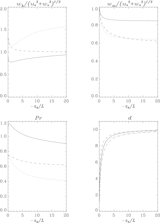
Fig. 6 Stability dependence of the surface velocity scales, Prandtl number (although I hope something is wrong with my coding of HB here!) and \(d\). Solid lines are from HB, dotted from the standard UM and the dashed from the revised formulation. The dash-dotted line for \(d\) is a potential modification, as described in the text.#
|
It is useful to compare the velocity scales in the revised scheme with those in the standard version, as well as those in Holtslag and Boville (1993), hereafter HB, on which the parametrization was originally based. Recall that HB and the standard UM set \(w_m = (u_*^3 + C_{ws} w_*^3)^{\frac{1}{3}}\) and \(w_h = w_m/Pr\), with \(C_{ws} = 0.6\) and 0.25, respectively, above the surface layer. The convective and neutral limits for \(w_h\) and \(w_m\) are given in Table 3 and the stability dependencies of several parameters are shown in Fig. 6. The parameter \(d\) in Fig. 6 contains the stability dependence of the gradient adjustment parameter:
The inclusion of an extra \(w_*/w_m\) factor in \(\gamma_{\chi}\) was a deliberate change by HB from the original Troen and Mahrt (1986) formulation on which the UM was based. This seems an appealing feature (HB’s \(\gamma_{\chi}\) will tend to zero as \(w_* \rightarrow 0\)) and probably should be considered for the revised scheme (the dash-dotted line in Fig. 6 sets \(d^{std} = 10 w_*^2/w_h^2\)). Similarly, \(f_2\) might benefit from an additional factor of the form \((V_{\mathrm{surf}}^3+ V_{\mathrm{Sc}}^3)/ V_{\mathrm{sum}}^3\) so that it too tends to zero in the neutral limit. Further analysis of LES and SCM tests will be required to verify this.
Note that the most significant change from the standard UM scheme is the change to \(w_h\) in the convective limit. Since \(\gamma_{\chi}\) remains unchanged in the convective limit, this reduction in \(w_h\) will result in a significantly smaller \(\overline{w'\chi'}_{ng}^{\mathrm{surf}}\) for the revised scheme which gives better agreement against LES.
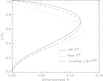
Compared to the standard scheme, it appears that the revised \(K_h^{\mathrm{Sc}}\) is very different. However, Fig.7 shows that this actually amounts to a small adjustment in the shape. In addition, note that the factors \(\varepsilon_h^{surf}\) and \(\varepsilon_h^{Sc}\) have been removed since the entrainment flux is now carried via the explicit \(f_2\) term.
Fig. 7 Standard UM \(K_h^{\mathrm{Sc}}\) (solid) and revised (dotted), both scaled by \(k z_h V_{\mathrm{Sc}}\). An upside-down version of \(K_h^{\mathrm{surf}}\) is also shown (dashed) for comparison.#
|
The blended scheme#
For high resolution simulations, the UM has a Smagorinsky-type subgrid
turbulence scheme, described in :umdp:028. However, this scheme is
only truly applicable for horizontal grid-lengths of order \(10\) m,
and any real-world simulation run at lower resolution than this will
inevitably have unresolved scales somewhere in the domain. Rather than
force the user to make an ad-hoc decision about the scales they are
interested in, and thus grid-length at which to switch from using the
boundary-layer parametrization (1D BL) to the subgrid turbulence scheme
(3D Smag), a method for blending the two parametrizations has been
developed. This blend is regime and scale dependent, allowing a single
parametrization to be used across resolutions, including the completely
unresolved/resolved extremes. This blending process is described in
Boutle et al. (2014), which gives some examples of its use
and comparison to simulations using either the 1D BL or 3D Smag schemes
only. Updated technical details from Boutle et al. (2014)
are reproduced below. Several options are available that are selected
using the switch blending_option. These all follow the same
principles but differ in their choice of what should constitute the
boundary layer and how to treat non-turbulent layers of the atmosphere.
As shown in Honnert et al. (2011), the rate at which turbulent structures become resolved appears to be different for different aspects of the flow. For example, moisture fluxes are on a larger scale than heat or momentum fluxes, and so transition to being sub-grid at lower resolution. This is just one of many challenges when creating a truly accurate grey-zone parametrization, and so our aim here is to start from the simplest possible approach which allows the model to transition from unresolved to resolved turbulence in a plausible way, without the user having to decide at which grid-length to switch from a 1D, non-local, to a 3D, local sub-grid scheme.
Given some function, \(W_{1D}\), which tells us how poorly resolved the turbulence is (\(=1\) if unresolved, \(=0\) if well resolved), we can use this to blend between the 1D BL and 3D Smag schemes. Both schemes have a local Richardson number formulation:
where \(K_\chi\) is the eddy diffusivity, \(l\) is the mixing length, \(S\) is the wind shear, \(f_\chi(Ri)\) is the stability function and \(\chi\) represents conserved heat and moisture variables, or momentum. Both schemes use the same stability function, and both schemes can use the full 3D shear for \(S\). Therefore the only difference is in the mixing length, which is calculated as
where \(l_{\mathrm{bl}}^{-1} = (\kappa z)^{-1} + \lambda_0^{-1}\) and \(l_{\mathrm{smag}}^{-2} = (\kappa z)^{-2} + (c_s \Delta x)^{-2}\), \(\kappa\) is the von Karman constant and \(c_s\) is the Smagorinsky constant. Near the surface \(l_{\mathrm{bl}}\) and \(l_{\mathrm{smag}}\) are identical, but the asymptotic values are different and this method weights the asymptotic value according to the weighting of the two schemes. For example, at \(\Delta x=1\) km, \(c_s\Delta x=200\) m (for \(c_s=0.2\)), whereas \(\lambda_0=\max(40\ {\mathrm{m}}, 0.15z_h)\), which allows for a small mixing length in shallow unresolved boundary layers (e.g. stable ones).
The Lock et al. (2000) scheme also contains a non-local component to the turbulent flux, and this is simply down-weighted by \(W_{1D}\) to ensure that it becomes less significant as the turbulence becomes better resolved. Therefore the full eddy diffusivity is given by
where \(K_\chi^{\mathrm{NL}}\) is the non-local diffusivity and \(l\) in Eq. (243) is given by \(l_{\mathrm{blend}}\) in Eq. (244). The turbulent flux is then calculated as
where \(F_\chi^{\mathrm{NL}}\) is the non-local flux. Therefore when \(W_{1D}=1\), the scheme of Lock et al. (2000) is recovered, whilst with \(W_{1D}=0\) the Smagorinsky-type scheme is recovered.
Now we need to define the function \(W_{1D}\) to blend the schemes. Within the boundary layer this is based on the turbulent kinetic energy partitioning given by Honnert et al. (2011). We choose the TKE partitioning because it is most closely linked to the eddy diffusivity we are trying to parametrize (for example a TKE based scheme would calculate the eddy diffusivity from the TKE), and simplify the function slightly, using
where \(z_{\mathrm{turb}}\) is the appropriate lengthscale of the turbulence, \(\beta\) is a scaling parameter which controls the speed of the transition from unresolved to resolved turbulence, \(r_f=\frac{1}{l_0-l_1}\), \(l_0=4\) and \(l_1=0.25\) (N. B. this formula is slightly modified from that given in [Boutle et al. (2014)]). Malavelle et al. (2014) demonstrated that this scaling method was applicable to any type of unstable boundary layer given an appropriate choice of \(z_{\mathrm{turb}}\). In Boutle et al. (2014) this functional form was applied everywhere, adjusting the values of \(z_{\mathrm{turb}}\) and \(\beta\) depending on the regime. The max function is present to force the lowest resolution simulations to just use the 1D mixing scheme. An alternative approach that differs above the boundary layer is described below.
The simplest case is for a well-mixed boundary layer, where the appropriate lengthscale is the boundary-layer depth (inversion height). Therefore we set \(z_{\mathrm{turb}}=z_h\), which is broadly consistent with Malavelle et al. (2014), and choose \(\beta=\beta_{\mathrm{bl}}=0.15\) to give the best match of our function to that of Honnert et al. (2011). These functions are shown in Figure 8(a) and are only dissimilar for small \(\Delta x\), where Eq. (245) tends to zero faster. This is by choice, to force the highest resolution simulations to use the 3D turbulence scheme.
Fig. 8 (a) Weighting for the 1D boundary-layer scheme as a function of \(\Delta x/z_{\mathrm{turb}}\), showing the function of Equation (245) (blue solid), the equation in Boutle et al. (2014) (black solid) and the TKE partitioning of Honnert et al. (2011) (mean thick dashed, 5th/95th percentiles thin dashed). (b) Schematic showing the calculation of \(z_{\mathrm{turb}}\) used in Eq. (245) for a well-mixed layer (black dotted) and a decoupled cloud layer (black solid).#
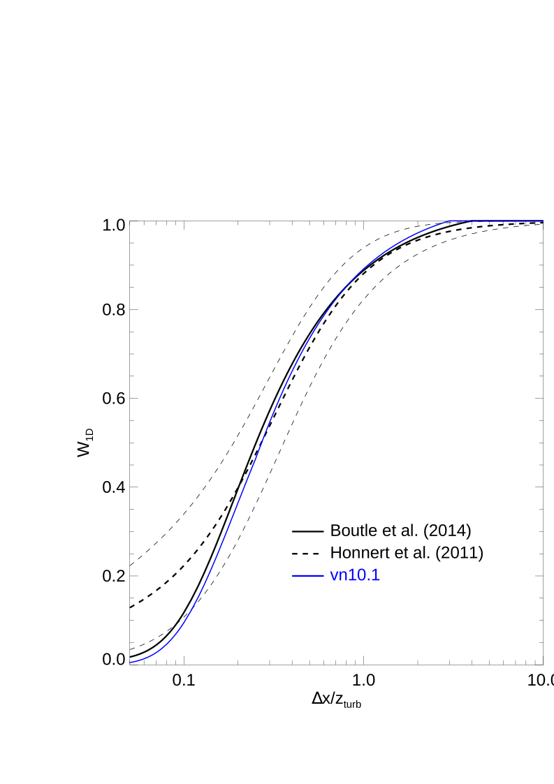
|
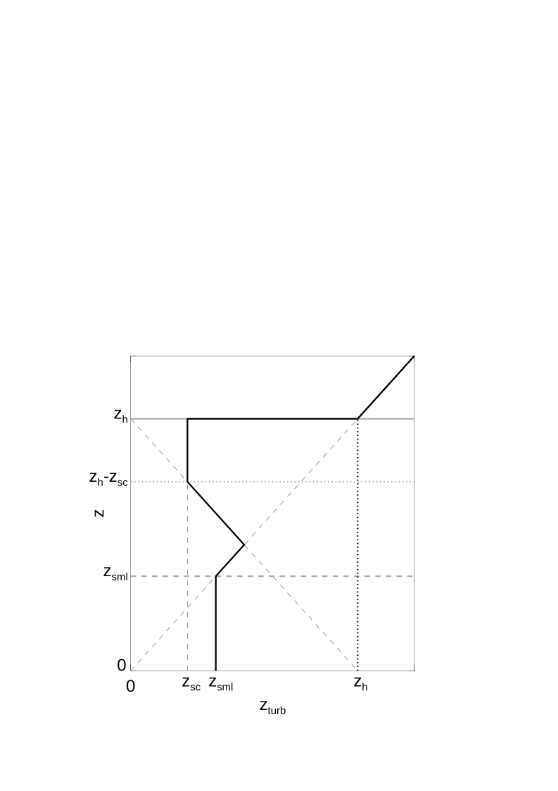
|
One of the key benefits of the Lock et al. (2000) scheme is its ability to represent decoupled stratocumulus layers, and this is a feature which needs to be maintained in the blended scheme. Physically they are similar to well-mixed surface driven boundary layers, and the Lock et al. (2000) scheme parametrizes them as such. The appropriate length scale is now the decoupled cloud mixed layer depth, \(z_{\mathrm{sc}}\) [i.e.~the depth through which a negatively buoyant parcel released at cloud top would descend, Lock (2001)]. In this case, below the decoupled cloud top we set
where \(z_{\mathrm{sml}}\) is the depth of the surface-based mixed layer
[i.e.~the depth through which a positively buoyant parcel
released at the surface would ascend, Lock et al. (2000)]. This is shown
schematically in Figure 8(b), and ensures that
\(W_{1D}\) has a high value in the poorly resolved surface mixed
layer and cloud layer, and a lower value in between those layers. Again,
this choice of \(z_{\mathrm{turb}}\) is broadly consistent with the
analysis of decoupled stratocumulus LES presented by
Malavelle et al. (2014). Finally,
Honnert et al. (2011) also included shallow cumulus
simulations and showed that the relevent length scale there was the
cloud top height. Most of the blending_option choices apply this to
all regimes diagnosed as cumulus-capped (see section Diagnosis of
boundary layer depth and type)
but alternatively (blending_option\(=\)4) this can be
restricted to strictly shallow cumulus clouds, defined as contiguously
cloudy levels (cloud fraction greater than SC_CFTOL) with cloud top
height below input parameter shallow_cu_maxtop. Note that the
diagnosis of shallow cumulus from the diagnosis parcel ascent (that was
used to identify a cumulus regime) was found frequently to indicate deep
convection even when the resolved clouds were shallow because the
diagnosis parcel, being undilute, would penetrate to the tropopause.
However, having decided the regime is shallow convection, we do still
set \(z_{\mathrm{turb}}\) to the diagnosis parcel top height because, for
current km-scale configurations (without a cumulus convection
parametrization), it was found that the resulting stronger parametrized
vertical mixing was beneficial for the development of the convection,
and that without this a widespread stratiform cloud layer could develop
instead.
Above the boundary layer top, Boutle et al. (2014) aimed for any free atmospheric mixing to be done by the 3D Smagorinsky scheme. Therefore, above the boundary layer top they use \(z\) as the appropriate length scale, and in general take \(z_{\mathrm{turb}}\) in Eq. (245) as the greater of that defined by (246) and \(z\). However, this did not give a particularly fast transition using the value of \(\beta_{\mathrm{bl}}\), therefore they used \(\beta_{\mathrm{fa}}=1\) at a height well above the boundary layer (\(z_{\mathrm{fa}}=z_h+1\) km), and transitioned between these regimes linearly using
However, because the above method still uses (245),
which depends on \(z_{\mathrm{turb}}/\Delta x\), the rate of transition
to 3D Smagorinsky with height above the boundary layer varies in an
undesirable way with grid size. It might be considered more logical to
think of non-turbulent regions of the free troposphere as unresolved
turbulence and so revert to the 1D mixing scheme there. An alternative
treatment(blending_option\(=\)3 or 4), then, is to increase
\(W_{1D}\) above the boundary layer top smoothly, to reach unity by
some physical height \(z_{\mathrm{fa}}\), to be independent of both
horizontal and vertical grid sizes. For
\(z_{\mathrm{turb}} < z < z_{\mathrm{fa}}\), then, we set
The cosine term in square brackets transitions smoothly from 2 at \(z=z_{\mathrm{turb}}\) to zero at \(z_{fa}\) where, although somewhat arbitrary, \(z_{\mathrm{fa}} = {\mathrm{min}}(2 z_{\mathrm{turb}}, z_{\mathrm{turb}}+1 {\mathrm{km}})\). The former term ensures the transition is well above any shallow boundary layers while the latter that it does not drift far into the free atmosphere. In addition, within any layers identified as turbulent, through having subcritical \(Ri\), \(z_{\mathrm{turb}}\) is set to the layer depth, in the same way as is done for decoupled stratocumulus in (246).
For current operational convection-permitting model grid sizes (1.5 km
in the UKV), the representation of cumulus convection remains a
challenge. One option is to include a grey-zone convection
parametrization, described in the documentation of that scheme (see
:umdp:027). Tests in the UKV, though, showed some detriment to the
spin-up of resolved scale convection (as well as somewhat poor
discrimination of precipitating versus non-precipitating parametrized
convection) that led to the development of an alternative strategy,
namely to abandon the blended turbulence scheme when pure cumulus
convection was diagnosed and leave the representation of cumulus
entirely to the resolved scales. This option
(blending_option\(=\)2) is also now discouraged.
Entrainment fluxes#
Summary: parametrized entrainment fluxes (at the top of mixed layers) are specified for momentum through an eddy-diffusivity, as described in section For momentum (and scalars if no subgrid inversion). For scalar variables, if the inversion is sufficiently sharp so as to be unresolved, the ideal is to specify the entrainment fluxes explicitly, as described in section Specification of entrainment fluxes in the 9B scheme, based on the subgrid inversion diagnosis described in section Diagnosis of a sub-grid inversion. Further details can be found in Lock (2001). If the profiles are such that the inversion is sharp but a subgrid inversion cannot be diagnosed, an eddy-diffusivity similar to that for momentum is used (see section For momentum (and scalars if no subgrid inversion)). If the inversion is thick enough to be resolved then an eddy diffusivity profile is constructed across the inversion (see section Resolved inversions) for both scalars and momentum fields. For tracer variables (scalars other than \(\theta_{\ell}\) and \(q_t\)), the entrainment fluxes are specified using an equivalent eddy-diffusivity, as described in section For tracers, when there is a subgrid inversion. Note that, as indicated below, several aspects of the implementation of entrainment fluxes were revised at the 9C scheme and these are documented separately.
The parametrization of the entrainment rate, \(w_e\) (given, in the absence of subsidence, by the rate of rise of the inversion), can be written (using the notation given in appendix Appendix: Definitions of the velocity scales)
where \(V_{\mathrm{sum}}^3= V_{\mathrm{heat}}^3+ V_{\mathrm{rad}}^3+ V_{\mathrm{br}}^3+ A_2 u_*^3\). The constant \(A_1\) is given a value 0.23, as in Lock (1998), and \(A_1*A_2=5\), as in Driedonks (1982). To allow for weak inversions, the Zilitinkevich (1975) correction is included in (247) with the constant, \(c_T=1\). A further parametrization for \(\alpha_t\), which is the fraction of the cloud-top radiative divergence (\(\Delta_F\), in Kms\(^{-1}\)) that occurs across the horizontally-averaged inversion in the LES, can be written
where the thickness of the inversion is parametrized as
\(\Delta z_i =
\mathrm{min}[V_{\mathrm{sum}}^2/\Delta b, 100]\) and \(L_{rad}\) is a
depth-scale for the radiatively-cooled layer (taken to be 15
\(\times
\,\mathrm{max}[200/z_c, 1]\), where \(z_c\) is the cloud depth). To
allow for a feedback with forcing of entrainment by buoyancy reversal
(see appendix Appendix: Definitions of the velocity scales),
\(\tilde{\alpha_t} = \alpha_t+ Br
(1-\alpha_t)\). following Lock (1998) and
Lock (2009). The calculation of the other
quantities required for (247) is described in
appendix Appendix: Definitions of the velocity scales. At
some point during the transition to a
decoupled boundary layer the surface-driven entrainment terms (the terms
in (247) proportional to \(V_{\mathrm{heat}}^3\) and
\(u_*\)) will no longer contribute to entrainment at cloud top,
because the two layers will have become entirely decoupled. If the
entr_smooth_dec switch is on then the surface contribution to the
parametrized entrainment at \(z_{\mathrm{h}}^{\mathrm{Sc}}\) is decreased
linearly as the \(\theta_{v\ell}\) difference between NTDSC and NTML
increases from 0.5 to 1K. The flag, COUPLED, is set to true and
\(z_{\mathrm{h}}^{\mathrm{Sc}}\) is used as the mixed-layer depth in
(247) as long as any surface-driven entrainment
remains. If the entr_smooth_dec switch is off then this transition
is discontinuous at a \(\theta_{v\ell}\) difference of 0.5K.
It should be noted that (247) takes no account of wind shear anywhere other than at the surface. How to quantify the shear generation of turbulence in DSC layers is not known. The direct impact of shear across the inversion is thought to be simply to diffuse the inversion in the vertical – this wind shear will contribute little to the mixed layer TKE and so can not contribute to the full process of mixing across the inversion and down into the mixed layer that is entrainment. However, important interactions between wind shear across inversions and cloud-top radiative cooling have been observed that are not yet accounted for in the UM.
The least well-determined part of (247) is the constant \(A_2\) – the constant in the Zilitinkevich correction, \(c_T\), is also approximate but is included to limit the growth of layers capped by weak inversions and for numerical safety. A further limit is applied to the value of \(w_e\) determined by (247) such that the inversion cannot rise by more than one grid-level in a timestep. With current vertical resolutions and timesteps this is not a serious restriction. The constants \(A_1\) and \(A_{\mathrm{br}}\) appeared to be determined within 10-20 % in Lock (1998), although only solid cloud sheets were simulated (as discussed further in appendix Appendix: Definitions of the velocity scales). Similarly the parametrizations of \(\alpha_t\) and \(\Delta z_i\) were found to be accurate but the parameter \(L_{rad}\) is currently only crudely represented in the UM.
Specification of entrainment fluxes in the 9B scheme#
Note that the 9C scheme (see next section) differs by generalising the approach to include all processes operating in the inversion grid-level, rather than just radiation.
If it is assumed that the turbulent fluxes reduce from their extremum at \(z=z_i\) (the ‘entrainment’ fluxes) to zero at \(z=h\) a small distance above, then \(\overline{w'\theta_{\ell}'}_{z_i}= - w_e \Delta \theta_{\ell}+ F|_h - F|_{z_i}\), so that
where the total heat flux \({\mathcal{H}} = \overline{w'\theta_{\ell}'}+ F_{\mathrm{net}}\) and \(F_{\mathrm{net}} = F- F|_{z_{\mathrm{b}}}\). The net radiative flux relative to the base of the mixed layers is simply calculated as
where NBDSC\(=1\) in SMLs, \({\mathcal{S}}_F\) are the temperature increments (in Ks\(^{-1}\)) from the radiation scheme and \(F_{\mathrm{net}}|_h\) is estimated by extrapolating down from \(F|_{z_{\mathrm{ \mathrm{NTML}}+\frac{3}{2}} }\) using the flux-divergence in grid-level NTML\(+2\) (and similarly for DSC layers).
The thermodynamic variables’ entrainment fluxes, then, are imposed nominally at the subgrid inversion height (\(z_i=\) \(z_{\mathrm{h}}\) and/or \(z_{\mathrm{h}}^{\mathrm{Sc}}\) ), diagnosed as described in section Diagnosis of a sub-grid inversion. The required grid-level fluxes (at \(z_{\mathrm{ \mathrm{NTDSC}}+\frac{1}{2}}\), for example) are then estimated using linear interpolation of \({\mathcal{H}}\) and \(\overline{w'q_t'}\) between \(z_{\mathrm{h}}^{\mathrm{Sc}}\) and the base of the mixed layer:
where \(z' = z-z_{\mathrm{b}}\), and similarly for the SML entrainment fluxes (at \(z=z_{\mathrm{ \mathrm{NTML}}+\frac{1}{2}}\)). The turbulent fluxes at the base of the mixed layer are assumed zero except for the SML where the surface fluxes are used. This interpolation is illustrated for a SML in Fig. 9.
Fig. 9 Idealised profiles of (a) \(\overline{w'q_t'}\) (dash-dotted line) and (b) \({\mathcal{H}}\) (dotted line), \(\overline{w'\theta_{\ell}'}\) (dash-dotted) and \(F\) (dashed). The continuous lines are the turbulent fluxes on the model grid indicated by the dashed horizontal lines.#
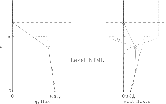
|
Note that, because (249) includes an explicit balance between the turbulent and radiative fluxes for \(\overline{w'\theta_{\ell}'}\), it is not possible to parametrize the entrainment fluxes through a single \(K_h\) for both \(\overline{w'\theta_{\ell}'}\) and \(\overline{w'q_t'}\). Furthermore, the radiative forcing of turbulence in the mixed layer is fixed through the timestep and so it is consistent to assume the entrainment fluxes (at \(z_i\)) are also fixed. Hence (249) are implemented explicitly, rather than via an eddy-diffusivity. This is discussed further, with reference to tracer fluxes, in section For tracers, when there is a subgrid inversion.
In order to allow for the long timesteps used in NWP and to facilitate movement of the subgrid inversion across grid-levels within a timestep, the parametrization of \(w_e\) and the model’s subsidence velocity, \(w_S|_{z_i}\), are used to calculate \(z_i\) at the next time-level (\(z_i^{n+1}\)). Currently, the latter is found by linear interpolation to \(z_i\) and both are assumed constant in time. If \(z_i^{n+1} < z_{\mathrm{ \mathrm{NTDSC}}+\frac{1}{2}}\), then the entrainment fluxes there (given by (249)) are multiplied by the fraction of the timestep that \(z_i\) was above this grid-level, namely \((z_i-z_{\mathrm{ \mathrm{NTDSC}}+\frac{1}{2}})/(z_i - z_i^{n+1})\). The full entrainment flux at grid-level NTDSC\(-\frac{1}{2}\) must then also be specified, given by (249) with \(z_{\mathrm{ \mathrm{NTDSC}}+ \frac{1}{2}}\) replaced by \(z_{\mathrm{ \mathrm{NTDSC}}- \frac{1}{2}}\). If \(z_i\) rises above \(z_{\mathrm{ \mathrm{NTDSC}}+\frac{3}{2}}\), the entrainment flux is specified only at this higher grid-level (multiplied by the fraction of the timestep that \(z_i\) is above this half-level) and the values of the mixed-layer \(K\) profiles are used in half-level NTDSC\(+\frac{1}{2}\) (these will be non-zero because \(z_i>z_{\mathrm{ \mathrm{NTDSC}}+ \frac{1}{2}}\)). Wherever the entrainment fluxes are specified explicitly, the eddy-diffusivities (both non-local and local) are set to zero. Also, the mean value of \(z_i\) during the timestep is used in (249) in order best to approximate the mean flux gradient across the mixed layer.
Finally, the entrainment flux is adjusted to allow for numerical entrainment arising from the model’s resolved vertical advection (as discussed in Lock (2001)). This is performed at whichever grid-level the entrainment fluxes are specified, to allow for any entrainment implied by a \(\theta_{\ell}\) subsidence increment, \(\Theta^{\mathrm{S}}\) (Ks\(^{-1}\)), at the model grid-level below. The subsidence increments could be obtained directly in the SCM but in the full 3D UM advection increments are dominated by the horizontal component. The subsidence increments are calculated, therefore, from the vertical velocity field using first order upwind advection (it would clearly be preferable to use the model’s actual vertical advection algorithm in the GCM although the errors incurred in this diagnostic calculation should not be very significant). The interpolated entrainment fluxes given by (249) are therefore calculated not using \(w_e\) but using an entrainment velocity, \(\tilde{w_e}\), that is reduced to allow for any subsidence increments applied to the grid-level below the entrainment flux. To take the case of \(z_{\mathrm{ \mathrm{NTDSC}}+\frac{1}{2}} < z_i^{n+1} < z_{\mathrm{ \mathrm{NTDSC}}+\frac{3}{2}}\) as an example, this reduced entrainment velocity is given by
with \(\tilde{w_e}\) constrained to lie between 0 and \(w_e\) and
Diagnosis of a sub-grid inversion#
The profile of \(\theta_{v\ell}\) is used to diagnose the height of a discontinuous inversion because it is approximately conserved under adiabatic vertical motion and is equal to the virtual potential temperature, \(\theta_v\), in the absence of cloud. This should ensure it is monotonically increasing with height in the statically stable free-troposphere of a GCM. If \(\theta_{v\ell}\) does not increase monotonically between grid-levels NTML and NTML+2 (or NTDSC and NTDSC+2), then entrainment fluxes are simply specified via (258) and none of the coupling with subsidence or radiation described above is attempted (the local scheme is also currently not set to zero above NTML or NTDSC when this occurs to allow it to diffuse out this static instability).
Fig. 10 Schematic illustrating the assumptions behind the subgrid diagnosis of \(z_i\).#
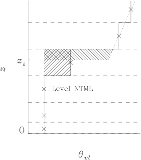
|
Having identified the model grid-level at the top of the well-mixed layer (either level NTML from the parcel ascent, as described in section The diagnostic parcel ascent and cumulus diagnosis, or NTDSC for DSC layers, see section Diagnosis of the vertical extent of the K-profiles– the analysis is the same for both), the grid-level above is designated the inversion level within which the diagnosis of a subgrid \(z_i\) will be made. It is assumed that \(\theta_{v\ell}\) in grid-level NTML\(+1\) represents a cell-average value. Thus, \(z_i\) can be calculated by assuming that the integral of \(\theta_{v\ell}\) over grid-level NTML\(+1\) for the model and for a profile with a discontinuous inversion at \(z_i\) are equal, as illustrated by the hatched areas in Fig. 10. To calculate the integral of the discontinuous profile, the lapse rate of \(\theta_{v\ell}\) between grid-levels NTML\(-1\) and \(NTML\), \(\gamma^{ \mathrm{ML}}\), is extended up to \(z_i\), while the stable lapse in the free atmosphere, between grid-levels NTML\(+2\) and NTML\(+3\), \(\gamma^{\scriptsize \mathrm{FA}}\), is extrapolated down. Equating these areas gives a quadratic equation in \(\Delta z_{disc} = z_{\mathrm{ \mathrm{NTML}}+\frac{3}{2}} - z_i\) which can be written
The coefficients are given by
Clearly, care must be taken to ensure that \(z_i\) is not only well-defined but also sensible (for example, as a rising inversion encounters more or less stable regions above). If \(b>0\) this suggests the estimated lapse rates are inappropriate and these are therefore set to zero and (251) is recalculated. The case \(c<0\) suggests the grid-level designated as the inversion level should have been considered as part of the mixed layer and so \(z_i\) is set to be fractionally below \(z_{\mathrm{ \mathrm{NTML}}+\frac{3}{2}}\) (i.e., as high as possible without attempting to diagnose a subgrid \(z_i\) in grid-level NTML\(+2\)). If \(b^2-4ac<0\) the quadratic equation has no real roots. In this instance \(z_i\) is set to fractionally below \(z_{\mathrm{ \mathrm{NTML}}+\frac{1}{2}}\) and NTML (and therefore the eddy-diffusivity profiles) is lowered by a grid-level. In all other circumstances, the required root is then \(\Delta z_{disc} = (-b - (b^2-4ac)^{1/2} )/(2a)\); the other root will either be larger or negative (if \(a<0\)).
In addition, from variations seen in \(z_i\) during single-column model simulations, the error in \(\Delta z_{disc}\) is estimated to be around 10% of the vertical resolution, \(\Delta_{\mathrm{ \mathrm{NTML}}+\frac{3}{2}} z\). Accordingly, if \(z_i\) is diagnosed as being less than \(z_{\mathrm{ \mathrm{NTML}}+\frac{1}{2}} + 0.1 \, \Delta_{\mathrm{ \mathrm{NTML}}+\frac{3}{2}} z\), NTML is lowered a grid-level and \(z_i\) is set fractionally below \(z_{\mathrm{ \mathrm{NTML}}+\frac{1}{2}}\). This small distance below the grid-level is taken to be \((\Delta t/2) \times 10^{-4}\) so that, were a small rate of rise of \(z_i\) (of \(10^{-4}\) ms\(^{-1}\), say) to be diagnosed, then \(z_i\) would spend at least half the timestep (of length \(\Delta t\)) in the next grid-level up. The specified fluxes would then contribute significantly to that grid-level’s evolution. Conversely, if \(z_i\) is subsiding, this technique allows the inversion to drop down a grid-level without requiring this to be detected by the initial parcel ascent.
Having calculated \(z_i\), the discontinuous jumps in \(\theta_{\ell}\) and \(q_t\) that are used in the entrainment calculation are calculated from similar integral assumptions:
with \(\chi = \theta_{\ell}\) and \(q_t\). Note that the lapse rate above the inversion has been ignored as there is no guarantee of monotonicity in \(q_t\) in the atmosphere above the inversion. In addition, (252) will become increasingly inaccurate as \(z_i\) tends to \(z_{\mathrm{ \mathrm{NTML}}+\frac{3}{2}}\) (and so \({\chi}_{\mathrm{ \mathrm{NTML}}+1}\) approaches \({\chi}_{\mathrm{ \mathrm{NTML}}}\)). Consequently, if the fraction on the right hand side of (252) is greater than 10, double grid-level jumps are used (i.e., \(\Delta \chi = {\chi}_{\mathrm{ \mathrm{NTML}}+2} - {\chi}_{\mathrm{ \mathrm{NTML}}}\)). Finally, note that (252) implicitly assumes the structure of the \(\theta_{\ell}\) and \(q_t\) profiles across the inversion grid-level are consistent with the diagnosed \(z_i\). This is very unlikely to be the case, for example, when running from an analysis so the 9C scheme uses what has been found to be a more robust algorithm, see the separate documentation.
It would clearly be advantageous to pass knowledge of this subgrid inversion structure to other parametrizations in the UM, particularly the cloud scheme as currently the cloud fraction in level NTML\(+1\) is essentially meaningless (being diagnosed from a mixture of cloudy boundary layer air and typically very dry free tropospheric air).
Specification of entrainment fluxes across sharp inversions in the 9C scheme#
As described in section Specification of entrainment fluxes in the 9B scheme, when the capping inversion is thinner than the model vertical grid it is important for the entrainment flux implementation that the subsidence increments are realistically and consistently distributed between the inversion grid-level and the mixed layer. Rather than work with the increments themselves, though, a more robust solution is to couple the subsidence and turbulent fluxes across the inversion, exactly analogously to the coupling of turbulent and radiative fluxes. This allows the total tendency of the inversion grid-level to be linked to whether the inversion should be rising or falling (determined from the balance between the parametrized entrainment rate, \(w_e\), and the large-scale vertical velocity evaluated at the inversion, \(w|_{z_h}\)).
Fig. 11 Subgrid (lines) and model (symbols) profiles and fluxes of, top row, \(q_t\) and, bottom row, \(\theta_{\ell}\): turbulent fluxes (dash-dotted, crosses), subsidence fluxes (dotted, diamonds), radiative flux (dashed, triangles) and total flux (solid, squares).#
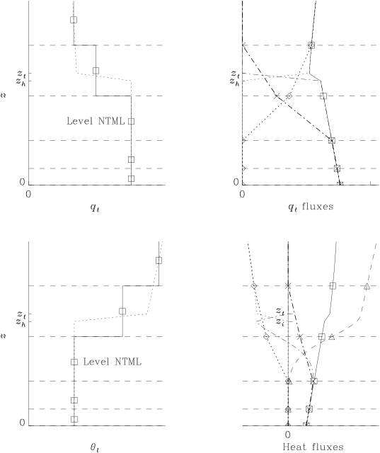
|
An idealised subgrid total flux profile is constructed from the parametrized entrainment flux and the increments from radiation, precipitation and subsidence, assuming a well-mixed boundary layer capped by a diagnosed subgrid inversion. The crucial step is to ensure that the total flux on the model entrainment grid-level equals the idealised total flux profile interpolated to that level. Consider the example illustrated in Fig. 11 of a well-mixed boundary layer up to \(\theta\)-level \(\mathrm{ \mathrm{NTML}}\). For the subgrid \(q_t\) profiles, the turbulent flux divergence generates a moistening across the inversion while subsidence generates drying. For this example it has been assumed the entrainment rate is slightly larger than the subsidence velocity at the inversion and so overall there is a weak moistening relative to the mixed layer (the total flux gradient is more negative across the inversion than in the mixed layer), consistent with the rising tendency of the inversion. For the model, the subsidence flux-divergence associated with the inversion is split across levels \(\mathrm{ \mathrm{NTML}}\) and \(\mathrm{ \mathrm{NTML}}+1\). To keep the net moistening of the model’s boundary layer and inversion consistent with the total subgrid flux profile, the model’s entrainment flux at \(\mathrm{ \mathrm{NTML}}+1/2\) (shown by the cross in Fig. 11) must be found by subtracting the subsidence flux at \(\mathrm{ \mathrm{NTML}}+1/2\) (diamond) from the total flux interpolated to \(\mathrm{ \mathrm{NTML}}+1/2\) (square). Exactly the same arguments follow for the \(\theta_{\ell}\) fluxes except that the situation is complicated by the addition of the radiative flux.
The above arguments can be generalised as follows. Writing \(F_{\chi}^{Tot}\) as the total flux of a conserved variable \(\chi\) (\(=q_t\) or \(\theta_{\ell}\)) and \(F_{\chi}^{NTP}\) as the flux from physics sources other than turbulence (i.e., radiation, \(F_{\chi}^{rad}\), in the above examples, but including precipitation fluxes, \(F_{\chi}^{ppn}\), in the full model) and \(F_{\chi}^{subs}\) as the flux from resolved scale subsidence, the total flux at the subgrid inversion height is given by:
As in section Specification of entrainment fluxes in the 9B scheme, (253) is derived by integrating the conservation equation for \(\chi\) over an inversion in which jumps occur over a thin layer with base at a height \(z_h\) and top at \(z_t\) (in the UM, the inversion is assumed to be infinitesimally thin so that \(z_t=z_h\)). This integration gives \(- w_e \Delta \chi = \overline{w'\chi'}|_{z_h} -(F_{\chi}^{NTP}|_{z_t}-F_{\chi}^{NTP}|_{z_h})\). Lock and Macvean (1999) related the non-turbulent flux divergence, \(F_{\chi}^{NTP}|_{z_t}-F_{\chi}^{NTP}|_{z_h}\), to radiative cooling occurring within undulations of the cloudy boundary layer top. Similar considerations need to be borne in mind when calculating all the non-turbulent fluxes in (253). First, the radiative flux is extrapolated down from \(\mathrm{ \mathrm{NTML}}+\frac{3}{2}\) to \(z=z_t\) using the divergence in the grid-level above the inversion as representative of the free-atmospheric divergence. Second, since the microphysical flux is generated within the cloud, \(F_{\chi}^{ppn}|_{z_t} = {F_{\chi}}^{ppn}_{\mathrm{ \mathrm{NTML}}+\frac{3}{2}}\). Finally, the subsidence flux-divergence across level \(\mathrm{ \mathrm{NTML}}\) and \(\mathrm{ \mathrm{NTML}}+1\) is assumed to be associated with the inversion so \({F_{\chi}}^{Subs}|_{z_h} = {F_{\chi}}^{Subs}_{\mathrm{ \mathrm{NTML}}-\frac{1}{2}}\). Thus, the finite-difference form of (253) becomes
Then, assuming a linear profile of \(F_{\chi}^{Tot}\) in the mixed layer, interpolating the total flux to the inversion flux grid-level gives
where \(z'\) (\(=z-z_{\mathrm{b}}\)) is height above the base of the mixed layer at \(z=z_{\mathrm{b}}\). Finally, the grid-level turbulent entrainment flux is given by:
This revised algorithm has several advantages over the previous. Firstly, the fluxes for \(q_t\) and \(\theta_{\ell}\) are coupled independently, whereas in the 9B version the coupling with subsidence was estimated using only the \(\theta_{\ell}\) increments in order to calculate \(\tilde{w_e}\) in (250). Secondly, this method makes it much simpler to include all processes, and precipitation in particular, in a consistent manner. Thirdly, since the total grid-level flux, \(F_{\chi}^{Tot}|_{\mathrm{ \mathrm{NTML}}+\frac{1}{2}}\) in (255), is used to calculate the entrainment fluxes, it is straightforward to ensure that the net budget of the inversion grid-level, namely \(- ( F_{\chi}^{Tot}|_{\mathrm{ \mathrm{NTML}}+\frac{3}{2}} - F_{\chi}^{Tot}|_{\mathrm{ \mathrm{NTML}}+\frac{1}{2}})/\Delta z\), is consistent with the entrainment/subsidence balance. In other words, to use \(\theta_{\ell}\) as an example, if the inversion is rising (falling) then \(F_{\chi}^{Tot}|_{\mathrm{ \mathrm{NTML}}+\frac{1}{2}}\) is limited to ensure that the inversion grid-level will cool (warm). Finally, if the inversion is rising we don’t want the inversion grid-level \(\theta_{\ell}\) to cool to less than \(\theta_{\ell}\) of the mixed layer by the end of the timestep. In other words, for \(\chi=\theta_{\ell}\), given
where the superscripts \(n\) and \(n+1\) refer to the model timestep, although strictly speaking \(n+1\) refers to fields after the boundary layer implicit solver. Requiring that \(\chi_{\mathrm{ \mathrm{NTML}}+1}^{n+1}\geq\chi_{\mathrm{ \mathrm{NTML}}}^{n+1}\) implies
The same arguments apply for \(q_t\), noting that the free atmosphere can be drier or moister than the mixed layer and so these cases must be treated separately. If \(\theta_{\ell}\) of the free atmosphere is colder than the mixed layer then no subgrid inversion treatment is attempted and entrainment is modelled using a straightforward eddy diffusivity.
Calculation of the inversion jumps in the 9C scheme#
In the 9B scheme, the discontinuous jumps in \(\theta_{\ell}\) and \(q_t\) that are used in the entrainment calculation were calculated from integral assumptions similar to those used to diagnose the subgrid inversion height, \(z_h\), and were given by (252). Note that \({\chi}_{\mathrm{ \mathrm{NTML}}+2}\) does not appear in (252) and so no direct information from the free atmosphere is used. Only if the budgets of \(\theta_{\ell}\) and \(q_t\) in level \(\mathrm{ \mathrm{NTML}}+1\) are entirely consistent with the rise and fall of the subgrid inversion will (252) give accurate results. This will not be the case during an assimilation cycle, for example, neither is it likely to be the case if the convection scheme is detraining into level \(\mathrm{ \mathrm{NTML}}+1\).
Instead, a more robust algorithm is used in the 9C scheme and the subgrid inversion calculation is only attempted where both \(\theta_{\ell}\) and \(\theta_{v\ell}\) are monotonically increasing and \(q_t\) is simply monotonic across the inversion. The formula used is:
subject to the constraint that the lapse rate adjustment should not reduce the two grid-length difference by more than half. The free-atmospheric lapse rates are given by
Calculation of the subsidence flux#
The vertical advection or subsidence flux, \({F_{\chi}}^{subs}\), is calculated by integrating estimates of the vertical advection increments. These estimates are made at 9B from the model’s vertical velocity field, \(w\), using first order upwind advection. As described above, however, the coupling between different flux profiles is performed on the model grid and, over land, these coordinate surfaces follow the underlying terrain. To correct this, the 9C scheme calculates the subsidence flux in grid-point, rather than physical space, by using \(\dot{\eta}\) (where \(\eta\) is the model’s vertical coordinate) rather than \(w\).
The following two examples illustrate why this represents an improvement. First, consider a boundary layer capped by a horizontal inversion in a horizontal flow over a rising land surface. Here \(w\) will be zero and yet the model will be generating a vertical advection flux across the inversion grid-levels, because \(\dot{\eta}\) is negative. Conversely, consider the same boundary layer but in a flow that follows the coordinate surfaces, going up and over a hill. Now there will be no vertical advection flux across the model’s inversion grid-level because \(\dot{\eta}\) is zero and yet \(w\) will be negative on the down-slope thus giving a spurious subsidence source to the 9B scheme.
Specification of entrainment eddy diffusivity#
As discussed above it is considered beneficial to specify the thermodynamic entrainment fluxes explicitly under the assumption that both the turbulence forcing and the inversion jumps change slowly compared to the timestep. Under the circumstance that no subgrid inversion can be diagnosed, not only is an alternative derivation of the entrainment fluxes required, but it is also deemed likely that these assumptions may be violated and so the entrainment fluxes are specified via an entrainment eddy diffusivity. Currently, this is also the case for momentum and tracer variables.
For momentum (and scalars if no subgrid inversion)#
For momentum, and scalars if a subgrid inversion cannot be diagnosed, see section Diagnosis of a sub-grid inversion, fluxes at the mixed layer top are specified through an eddy diffusivity which is given by
noting the Charney-Philips grid implying stresses are staggered from scalar fluxes. The Prandtl number, \(Pr\), takes the same form as for the non-local \(K\) profiles, see section The non-local scheme.
Substituting (258) in (212) gives, for example, \(\overline{w'\theta_{\ell}'}|_{\mathrm{ \mathrm{NTML}}+\frac{1}{2}} = - w_e \Delta_{\mathrm{ \mathrm{NTML}}+1} \theta_{\ell}\). Note that this gives entrainment buoyancy fluxes identical to (248) as long as there is no buoyancy reversal generation of turbulence (i.e.,\(V_{\mathrm{br}}=0\)) and if variations in the grid-level jumps across the timestep are ignored. The former is because the other terms in (247) are inversely proportional to \(\Delta b\). The latter will never actually be true and can give rise to large errors if the inversion is rising quickly. Therefore, the thermodynamic entrainment fluxes are specified explicitly where possible.
The advantages of diagnosing the subgrid inversion are that it allows consistency between the turbulent and radiative fluxes and large-scale vertical advection, it reduces grid-resolution errors arising from the mixed layer depth calculation and it allows a more accurate calculation of \(V_{\mathrm{br}}\) and \(\alpha_t\). For momentum, because the jumps across inversions are typically small and variable, it seems unwise numerically to attempt to specify the inversion stresses explicitly and so (258) is always used. For the 9C version, the entrainment \(K_m\) given by (258) is imposed at the height of the temperature inversion \(z_{\mathrm{h}}\) (either subgrid or at \(z_{\mathrm{ \mathrm{NTML}}+\frac{1}{2}}\)) and \(K_m|_{\mathrm{ \mathrm{NTML}}+\frac{1}{2}}\) is calculated from (234) and (237), noting the use of the \({\mathcal{E}}\) factors.
Resolved inversions#
An inversion is defined as being resolved when it extends above the flux-level above the usual entrainment interface level (see section Diagnosis of inversion thickness), i.e. when
When this happens, there is no subgrid inversion diagnosis and the entrainment parametrization follows the methodology given in section For momentum (and scalars if no subgrid inversion) to give \(K_h|_{\mathrm{ \mathrm{NTML}}+\frac{1}{2}}\). The diffusion coefficient profile within the inversion is then calculated assuming the \(\theta_{v\ell}\) flux profile within the inversion decreases following a cosine shape from the standard parametrized entrainment flux at the inversion base to zero at the inversion top, i.e.:
where \(z'=(z-z_{\mathrm{h}})/\Delta z_i\) is scaled height within the inversion. This flux profile is then converted into a diffusion coefficient profile by inverting the standard flux parametrization:
The diffusion coefficient for momentum entrainment is calculated in the same way, allowing for the staggered grid, with the same \(Pr\) as in (258).
For tracers, when there is a subgrid inversion#
Here ‘tracers’ refers to scalar variables other than \(\theta_{\ell}\) and \(q_t\): aerosols, \(q_f\), etc. Ideally, tracer entrainment fluxes would be specified explicitly in the same way as for \(\theta_{\ell}\) and \(q_t\). However, specifying the entrainment flux effectively specifies the net change in mixed-layer tracer concentration across the timestep. Thus, if the mixed-layer tracer concentration is small at the start of a timestep and the entrainment flux is larger than the surface flux, the mixed-layer concentration could go negative (and tests indicated that this did indeed happen). Specifying the entrainment flux assumes that both the turbulence forcing and the inversion jump change slowly compared to the timestep. Whilst this is true for atmospheric \(\theta_{\ell}\) and \(q_t\), the latter is not true for tracers with a small boundary layer concentration. Consequently, for a tracer field \(\chi\), the parametrized entrainment fluxes \(\overline{w'\chi'}_{ z_{\mathrm{ \mathrm{NTML}}+\frac{1}{2}} }\) are calculated from (249) but are implemented through an equivalent entrainment eddy-diffusivity given by:
Note from (212) that (260) gives the parametrized flux if \(\Delta_{\mathrm{ \mathrm{NTML}}+1} \chi\) does not change across the timestep (see section Implicit solution of the diffusion equation for a description of the implicit numerical solution of (207)). As (260) involves the potentially numerically dangerous calculation of \(\Delta \chi/\Delta_{\mathrm{ \mathrm{NTML}}+1} \chi\) (where \(\Delta \chi\) is the subgrid inversion jump, given by (252)), the following constraints are also ensured:
Surface Exchange#
Note that the surface scheme itself is documented under the JULES documentation.
The theoretical basis.#
Making the assumption that Monin-Obukhov similarity theory for the surface layer is valid the gradients of model variables in the surface layer are related to the surface fluxes by:
where subscript 0 represents a surface value and subscript * represents a surface layer scaling quantity. \(\phi _{m}\) and \(\phi _{h}\) are the Monin-Obukhov stability functions (for the form of these see section 8.3 below). \(L\) is the Monin-Obukhov length scale defined by
where F\(_{B0}\) is the surface buoyancy flux defined by
The buoyancy coefficients in equation (265) are given in appendix Appendix: Derivation and definitions of the buoyancy parameters with the subscript 1 denoting a value at the lowest level in the atmosphere model.
Equations (261)-(263) can be integrated from the “surface”, i.e. the roughness height where the surface variables are defined, to a reference height in the surface layer, for modelling applications, the height, z\(_{1}\), of the bottom model layer above the surface. The resulting expressions for the surface turbulent fluxes are:
where \(\Delta\)X=X\(_{1}\)-X\(_{0}\). From (266) and (267) the surface buoyancy flux in definition (264) is
The surface exchange coefficients in equations (266)-(268), c\(_{D}\) and c\(_{H}\), are given by
where
z\(_{0m}\) and z\(_{0h}\) are the surface roughness lengths for momentum and scalars respectively.
The equations for the surface turbulent fluxes, (266)-(268), can be written in the forms
where the effective wind speed for surface turbulent exchanges, \(V\), is defined by
and the surface conductances for scalars and momentum are respectively
The surface exchange coefficients can then be written in any of the following forms:
In order to close the system the surface scaling velocity, v\(_{\ast }\), needs to be specified. If
we have the standard Monin-Obukhov theory and it is easy to deduce that with this definition \(v_{\ast } = c_{D}^{1/2} \Delta\)v and V=\(\Delta\)v. To allow for the effect of turbulent and cloud-scale gusts on the surface turbulent fluxes the surface scaling velocity, v\(_{\ast }\), can be defined as
The second term represents the effects of turbulent eddy-scale convective gusts and w\(_{\ast }\) is the turbulent convective scaling velocity defined by
for F\(_{B0} >\) 0 and zero otherwise. z\(_{i}\) is the height of the top of the surface-based turbulent mixing layer. \(\gamma _{t}\) is a dimensionless constant which can be determined empirically or tuned within empirical limits. The third term represents the effects of deep convective cloud-scale gusts; the inclusion of this term is optional. The form implemented is taken from Redelsperger et al. (2000), in which the velocity scale, w\(_{c}\), is a function of the convective downdraught mass-flux at cloud base. (Note that the published expression is given as an adjustment of the 10-m wind and has been scaled to make it consistent with \(v_\ast\).) A further term \(\gamma _{m}^{2}\)w\(_{m}^{2}\) could be included in low resolution models to represent the effects of mesoscale gusts but this is not done in the Unified Model. The low wind speed limit, i.e. as \(\Delta\)v \(\to\) 0, for unstable conditions (with w\(_{c }\)= 0) can be seen to be
which implies that
Thus the low wind speed limits for the sensible and latent heat fluxes are obtained by substituting (286) into (266) and (267) with the surface transfer coefficients evaluated with L given by (287). The finite limit for L implies that the form of the stability functions, \(\phi\), for very large and negative \(\zeta\) is unimportant. However, the value of \(\Phi_{h}\) for L given by (287) is needed if the value of \(\gamma _{t}\) is determined from measurements of say the latent heat flux in very low mean wind conditions.
Comparison with the Godfrey and Beljaars (1991) formulation for gustiness#
We can define the mean gust speed at height z\(_{1}\) by
Using the definitions of \(V\) (278) and \(v_{\ast }\) (284) it can be deduced that
where
Thus in this formulation the mean gust speed is a function of height above the surface through the same factor, \(\Phi _{m}\)(z), which determines the profile of the mean wind v in the surface layer (see Eq. (268)). The values of \(\Delta\)v, v\(_{g}\) and \(V\) thus tend to zero as z \(\to\) 0. Note that v\(_{g} \to\) W\(_{g}\) as \(\Delta\)v \(\to\) 0 and that v\(_{g} \to\) 0 as the convective gustiness scaling velocities tend to zero.
Equation (288) can be rewritten as
which is exactly the form of Godfrey and Beljaars (1991). However Godfrey and Beljaars (1991) define the mean gust speed as \(\beta\)w\(_{\ast }\). Thus they directly modify the mean surface to air wind difference, \(\Delta\)v, with the gustiness or turbulent convective scaling velocity, w\(_{\ast }\), combining a grid dependent quantity with a constant scaling speed. The two formulations are similar in that they introduce a mean gust speed but differ in their assumption about whether this has a non-constant profile in the surface layer. Although transitory wind gusts may not be as close to equilibrium with the surface characteristics as the mean wind they should have a profile in the surface layer which approaches zero at the surface (strictly at the roughness height z\(_{0m})\).
The two formulations can be made equivalent by assuming that Godfrey and Beljaars (1991) \(\beta\) is not constant but is given by \(\gamma _{t}(\Phi _{m}\)(z)/k) which tends to zero as the surface is approached. However, over sea points where the roughness length is small (of order 10\(^{-4}\) m) and for which Godfrey and Beljaars (1991) derived their formulation, \(\Phi_{m}\)(z) varies at most by about 15% between 10 m and 50 m. Assuming a constant \(\beta\) does not lead to much inaccuracy in these circumstances. If gustiness is included over land, as is the case in the Unified Model, the higher roughness lengths lead to a greater variation in \(\Phi _{m}\)(z) in the region where models generally have their lowest level placed.
If \(\gamma _{t}\) = 0.08 then in the low wind speed limit of an unstable tropical maritime surface layer with a virtual temperature lapse of 1.5 K, a specific humidity lapse of 7x10\(^{-3}\) kg/kg, SST=303.16 K and a boundary layer depth of 800 m we obtain a latent heat flux of 37.08 W/m\(^{2}\) assuming the form for the stability functions given below.
Making surface exchange consistent with flux differencing#
The boundary layer scheme increments conserved quantities using differences in fluxes across a layer. This is strictly consistent only if the conserved quantity is a mass-weighted mean across the layer, rather than a representative value, such as the value at the middle of the layer. If the profile of the conserved quantity is linear the mean of the quantity is the same as the point-value in the middle of the layer, but this is not so if the profile is not linear. Near the surface, the profiles will be logarithmic in neutral conditions and so the values in the middle of the layer will be larger than the mean values. Surface similarity in the UM is applied treating taking the wind and temperature in the bottom layer as point values in the calculation of surface fluxes and is therefore not absolutely consistent with flux differencing. Whilst the effect of this difference is not large, it is desirable to have the option of correcting it, which is done by enabling the option to “make surface exchange consistent with flux differencing.” The following discussion explains how this is done.
In effect, the UM takes the displacement height for momentum as \(-z_{0m}\), where \(z_{0m}\) is the momentum roughness length. The profile of wind is therefore determined by Monin-Obukhov theory as
with \(u_*\) being the friction velocity, \(L\) the surface Obukhov length and \(\phi_m\) the similarity function. It is common practice to introduce a new function \(\psi_m\) such that \(\phi_m(\zeta)=1-\zeta \partial \psi_m / \partial \zeta.\) Redefining the vertical coordinate as \(\zeta=z/L\), we have
This is also frequently written as
The mean over the lowest layer, of depth \(z_1\) (or \(\zeta_1\) in the rescaled coordinate), is therefore
We consider the three terms within the integral separately. For the first,
For the second,
\(\phi_m-1\) is retained in the last integral since this will prove convenient in later algebra. The third integral is trivial. Hence,
Thus, in practical terms, the standard function \(\Phi_m\) is evaluated at the top of the layer, scaled by \(1+\zeta_{0m}/\zeta_1\) and reduced by the mean value of \(\phi_m\). For standard Monin-Obukhov functions, this last integral is easy to perform. In the limit \(L \rightarrow \infty\) it becomes 1 and to avoid a numerical singularity it is set equal to 1 in this (nearly neutral) limit. The adjustment of the thermal Monin-Obukhov function is exactly equivalent.
Algorithmically, the existing routine PHI_M_H is replaced by
PHI_M_H_VOL which takes the same inputs except that the heights are
the top of the layers. This is done when the surface fluxes, or
turbulence scales \(u_*\) and \(\theta_*\) are calculated.
Monin-Obukhov functions are also used to calculate winds and
temperatures at observed levels. In this case a value at a particular
height is required, so the existing Monin-Obukhov routine should be
used.
The form of the stability functions.#
For stable conditions, i.e. \(\Delta\)B \(\ge\) 0, the stability functions are given by Beljaars and Holtslag (1991):
where \(\zeta _{1}\) = (z\(_{1}\) + z\(_{0m})\)/L, \(\zeta _{0m}\) = z\(_{0m}\)/L, \(\zeta _{0h}\) = z\(_{0h}\)/L and
with \(a = 1\), \(b =2/3\), \(c = 5\), \(d = 0.35\).
Note that the bulk flux Richardson number for the surface layer is given by
so the Beljaars and Holtslag (1991) functions imply Ri\(_{f B} \to\) 1/a = 1 as z\(_{1}\)/L \(\to \infty\).
For unstable conditions, i.e. \(\Delta\)B \(<\) 0, the Dyer and Hicks forms [Dyer (1974)] are used:
(Note that \(\phi _{h}\prime\) is discontinuous at 0.) These are only empirically verified for \(\zeta \ge\) -1. Evaluating the integrals (273) and (274) we obtain:
where
and
where
The iterative algorithm for calculating the surface exchange coefficients#
For conditions that are stable, i.e. \(\Delta\)B \(\ge\) 0, or near-neutral (taken as \(\Delta\)v \(\ge\) 2 ms\(^{-1}\)), then start the iteration from the neutral limit, so
Otherwise (if \(\Delta\)B \(<\) 0 and \(\Delta\)v \(<\) 2 ms\(^{-1}\) ) start from the greater of the neutral and convective limits for \(v_\ast^{(0)}\), so
Then calculate
Having set up initial values the iteration loop can be entered (this is the original method used but contains an inconsistency in the treatment of boundary-layer convective gustiness, as described in section 8.4.1):
DO n = 1 to N
END DO.
For neutral and stable conditions (\(\Delta\)B \(\ge\) 0) start the iteration from the neutral values and set w\(_{\ast }\)=0 in the above iteration loop.
Use the final (N) values of C\(_{H}\) and C\(_{D}\) to calculate the surface sensible and latent heat fluxes and surface stress:
N is the last iteration value. N = 5 is currently used.
For sea points the momentum roughness length and the wind mixing energy flux are calculated from v\(_{\ast }^{(N)}\) using the formulae in subsection 8.6 below.
Correction to the iterative algorithm#
The above implementation of boundary-layer convective gustiness in the Monin-Obukhov iteration contains an inconsistency. The overall effect turns out to be small, but it is desirable to use the corrected form, which is derived as follows.
We decompose the wind as \({\mathbf{u}}=\bar{\mathbf{u}} + {\mathbf{u}}_g + {\mathbf{u}}'\), representing, respectively, the large-scale, gust and small-scale turbulent contributions to the velocity. Locally, Monin-Obukhov theory then gives
We ignore the spatial variation of \(\Phi_m\), expecting that the principal effect of locally stronger winds is to increase the local stress - this is exactly true in nearly neutral flow. The local stress is aligned with the wind so
With the assumption that \(\Phi_m\) does not vary spatially,
where \(C_D\) is the standard drag coefficient, \(\frac{k^2}{\Phi_m^2}\). The grid-box mean effect is
which is the product of the enhanced wind speed (including gusts) and the mean velocity. The magnitude of the stress is then \(\langle\tau\rangle = \rho C_D S U\), with the last two symbols representing the mean wind speed, including gusts, and the mean background velocity.
In the model, we want to write this as an effective drag coefficient, \(C_{De}\), so that \(\langle\tau\rangle = \rho C_{De}U^2\). Now define \(\tilde u_* = \frac{k}{\Phi_m}U\), the friction velocity due to large-scale flow, and \(\hat u_* = \frac{k}{\Phi_m}S\), the friction velocity due to the total flow, including gusts (again implicitly assuming that \(\Phi\) is unaffected by the gusts). The representation is \(\hat u_*^2 = \tilde u_*^2 +\gamma_t^2 w_*^2\). Then,
The variable CDV in the routine FCDCH within the Monin-Obukhov
iteration will then be \(\frac{k}{\Phi_m}{\hat u_*}\) (note that it
is divided by \(U\) at the end of the routine). This is indeed coded
at the end of the loop; but in the original code CDV is used to
calculate \(\tilde u_*^2\) at the beginning of the routine. In fact,
\(\tilde u_*^2 = (k/\Phi_m)\tilde u_* U\), which differs from the
coded result by a factor of \(\tilde u_*/\hat
u_*\). After this step, the purported \(\tilde u_*\) is augmented by
the gust contribution to get \(\hat u_*\). This has the consequence
of overestimating \(C_{De}\) and also means that what is described
as U_S in this loop is not \(\tilde u_*\), but
\(\sqrt(\tilde u_* \hat
u_*)\).
If we let \(v=\sqrt(\tilde u_* \hat u_*)\), then we get
In the corrected version this expression is used to calculate V_S,
namely \(\hat u_*\) within the iteration.
The interpolation of surface layer variables to standard observation heights#
Integrating (263) between the roughness height, z\(_{0m}\), and the observation height z\(_{ob}\) we obtain
Using the expression for the surface turbulent stress this gives the interpolation formula
For wind z\(_{ob}\) is set to 10m and the last iteration (N) values of C\(_{D}\), L and \(v_{\ast }\) are used. Integrating (261) and (262) between the roughness height, z\(_{0h}\), and the observation height z\(_{ob, }\) we obtain for the scalar \(X\) (\(=T+(g/c_{P})z\) , \(q\) or tracer amount)
and using the expression for the surface flux \(F_{X0}\) of the scalar quantity \(X\) this gives the interpolation formula
For temperature and humidity z\(_{ob}\) is set to the screen height (1.5 m) and the last iteration (N) values of C\(_{H}\), L and \(v_{\ast }\) are used.
The parametrization of decoupling#
In the foregoing analysis it is tacitly assumed that the surface layer, up to the model’s lowest grid level, is in equilibrium with the surface and lies within the constant flux layer. In light winds, and when the surface temperature falls quickly, these assumptions are invalid; equation (327) then yields temperatures at the height of observation that are too closely tied to the surface temperature. Observed temperatures may be significantly warmer: this may be termed decoupling. Two parametrizations of this effect are available. Both involve the idea that as the wind becomes very light radiative cooling comes to determine the temperature profile.
The first parametrization simply sets the interpolation coefficient between the surface temperature and that on the model’s lowest level according to the radiative equilibrium profile when the Richardson number exceeds 0.25 (a typical criterion for high stability).
The second more elaborate scheme is directed at the evening transition, when the surface temperature is falling rapidly: it is under such conditions that the impact of decoupling on the air temperature is greatest. For a couple of hours after the surface temperature drops below the air temperature, radiative cooling directly to the surface largely determines the atmospheric cooling rate when the wind is light and this may easily be calculated, provided that a parametrization of the transmission between the air and the surface is available: this parametrization depends on the absorbing properties of atmospheric trace gases. Explicitly, we have
where \(\dot T_{ob, \mathrm{ rad, surf}}\) is the cooling rate of the air at the height of observation due to direct radiative exchanges with the surface, \(T_{ob}\) is the air temperature at that height, \(T_s\) is the temperature of the surface and \({\mathcal{K}}(z_{ob})\) depends on the concentration of trace gases in the atmosphere, in practice water vapour and carbon dioxide, and their spectroscopic properties. The contributions of water vapour and carbon dioxide are, to a good approximation, additive, so we may write
where \(q_w\) and \(q_c\) are the specific concentrations of water vapour and carbon dioxide and \(\mu_w\) and \(\mu_c\) are the respective pathlengths between the observation height and the surface. The functions \({\mathcal{C}}_w\) and \({\mathcal{C}}_c\) are parametrized and explicit functional forms are included in the code.
In stronger winds turbulent cooling will be more important, so the scheme must approach the standard procedure in that limit. Within the context of local scaling, it can be shown that the depth of the atmosphere which feels the impact of surface cooling must scale on \({\mathcal{L}}=(u_*^3/ (g/T_s)\dot T_s)^{1/2}\), where \(u_*\) is the surface friction velocity, \(\dot T_s\) is the surface cooling rate. This parameter is used as a measure of the strength of turbulence to define the relaxation back to the strong-wind limit.
To implement the scheme, the liquid-frozen potential temperature at the height of observation, \(\theta_{ob}=T_{ob}+(g/c_P)z_{ob}-(L/c_P) q_{cl} - ((L+L_f)/c_P) q_{cf}\) is made a prognostic. Whenever the surface buoyancy flux changes sign and becomes stable, this prognostic is initialized using standard theory. On subsequent timesteps, it is updated to allow for radiative cooling to the surface, giving a provisional value \(\theta_{ob}'\), and then relaxed back towards the result that would be obtained from standard similarity theory, \(\theta_{ob, \mathrm{ sim}}\), as in the last section:
By tuning against an idealized highly vertically resolved model based on local scaling we set,
with
The explicit dependence of \(W\) on the timestep, \(\delta t\), ensures that the results converge as \(\delta t \rightarrow 0\). The exponential factor involving the Coriolis parameter, \(f\), is intended to represent the recoupling of the surface and atmosphere as growing directional shear at the top of the incipient stable boundary layer generates turbulence. This factor is somewhat exaggerated relative to the results of the model against which it is tuned, as a cautionary measure to ensure that decoupling is not allowed to persist too long after the transition. This is the purpose of the inclusion of the factor \(0.4 f t_{\mathrm{ trans}}\), where \(t_{\mathrm{ trans}}\) is the time since the transition.
It must be stressed that these schemes are heuristic and that the precise behaviour in weak turbulence is not fully understood. The second scheme appears to work well during the evening transition, but for reasons of caution decoupling is suppressed somewhat too rapidly. The simpler first scheme underestimates decoupling during the transition, but allows it to persist longer, although tending to overestimate it on these timescales. Overall, the second scheme is to be preferred.
The surface fluxes for sea and sea-ice gridboxes#
For gridboxes with sea-ice (i.e. where sea-ice fraction, f\(_{I} >\) 0) sensible and latent heat fluxes are calculated separately for the sea and ice parts of the gridbox and combined with appropriate weighting to obtain the total fluxes into the atmosphere. This is done because the two surfaces can have very different temperatures and also differ in their roughness.
The sea and sea-ice surface fluxes of sensible heat, moisture and momentum are calculated using gridbox mean surface transfer coefficients, \(<\)C\(_{H}>\) and \(<\)C\(_{D}>\). These are linear combinations of the corresponding coefficients calculated for the ice-free sea (L), typical Marginal Ice Zone broken sea-ice (MIZ) and complete ice cover (I).
The surface sensible heat and moisture fluxes are calculated separately for the ice-free (leads) and ice-covered parts of the gridbox. Although the fluxes over the two surfaces are calculated from gridbox mean surface transfer coefficients, the different surface temperatures give different fluxes. The ice surface temperature is predicted from a surface energy balance and ice heat conduction model (see the documentation for the land and ice surface processes component of the Unified Model). In current versions of the model the sea surface temperature (SST) is assumed to be 271.35 K, the freezing point of sea water, whenever the ice fraction is greater than zero. This is unrealistic except for genuine leads (i.e. large ice fraction) and a future version of the model will allow the SST to be larger than 271.35 K for gridboxes with sea-ice.
The wind mixing energy flux, F\(_{WME}\) , is the rate of production of turbulent kinetic energy per unit area in the sea surface layer by the wind stress at the air-sea interface. In atmosphere-only configurations of the Unified Model this quantity is a useful diagnostic. When the atmosphere model is coupled to an ocean model the wind mixing energy flux is accumulated over an ocean model timestep and then used in the calculation of the mixing in the upper layers of the ocean. The gridbox mean wind mixing energy flux is given by
where \(v_{\ast }\) is calculated using the drag coefficient for the leads part of the gridbox, c\(_{D(L)}\), rather than the gridbox mean value, \(<\)c\(_{D}>\), when there is partial ice cover.
Roughness Lengths over the Sea#
The roughness lengths for momentum and scalars depend on both the atmospheric flow and the wave state. The dependence on wave state is not fully understood and is still a subject of active research. In any case, it could only fully be represented in a coupled wave-atmosphere model. Simpler more empirical schemes are therefore currently used in the Unified Model.
In all schemes available here the momentum roughness length is given by
which is a generalisation of Charnock’s formula to include low-wind conditions [Smith (1988)]. \(\alpha\) is Charnock’s coefficient, which is determined from field measurements. It is often taken as a constant, but more elaborate schemes include a dependence on wind speed. In practice the difference between different parametrizations of the momentum roughness length therefore comes down to the specification of Charnock’s coefficient.
There is greater uncertainty in the roughness lengths for scalars and the dependencies are described separately for each scheme. Note that whilst the full versions of some schemes prescribe different roughness lengths for heat and moisture, in the Unified Model we have only a single roughness for all scalars.
Schemes are selected by setting the variable iseasurfalg, as now described.
Option iseasurfalg=0. The original and most basic scheme comprises a fixed value of Charnock’s coefficient and a fixed scalar roughness length. Typical values of Charnock’s coefficient lie in the range 0.011-0.018 and a typical value of the thermal roughness length is \(z_{0h(sea)}\) = 4x10\(^{-5}\) m.
Option iseasurfalg=1. The use of a fixed thermal roughness length, as above, leads to a rapid increase in the exchange coefficient for moisture as the wind speed increases that is at variance with observational evidence. A parametrization of the scalar roughness length was developed from surface divergence theory [Csanady (2001)], as described by Edwards (2007). This involves an inverse dependence of \(z_{0h}\) on the friction velocity in the aerodynamically smooth limit and an inverse dependence of \(z_{0h}\) on \(z_{0m}\) at higher wind speeds that reduces the increase in the exchange coefficient with wind speed.
During iteration of the equations of surface transfer to calculate the Obukhov length, the friction velocity changes, so implicitly changing the roughness lengths. Historically, in the algorithm adopted in the Unified Model,roughness lengths have not been modified within this iteration, with values from the previous timestep being used. The scheme was therefore originally implemented in a form that was based on conditions at the previous timestep, but did not require adding \(z_{0h}\) to the dump. To cope with conditions of light winds, this required an iterative calculation of \(v_\ast\) from \(z_{0m}\) from the previous timestep before the calculation of the Obukhov length and \(v_\ast\). Note that although there is not a 1-1 relationship between \(v_\ast\) and \(z_{0m}\), the ambiguity is in practice removed by the consideration that the inversion is only of relevance in conditions of light winds.
With this scheme a fixed value of Charnock’s coefficient must be specified as above.
Option iseasurfalg=2. An alternative version of the foregoing scheme has been developed that includes full iteration of the roughness lengths within the iteration for the Obukhov length.
Option iseasurfalg=3. This option provides various forms of the COARE algorithm. The COARE algorithm exists in various forms and continues to be developed. Version 3.0 [Fairall et al. (2003)] has been extensively used, while version 3.5 [Edson et al. (2013)] has recently been released. Whilst the full COARE algorithm provides a complete description of surface transfer at the sea surface, here we use only the expressions for the roughness lengths.
In current versions of the scheme Charnock’s coefficient is specified using a linear relationship between the 10-m wind speed, valid over a certain range of wind speeds, with fixed values outside the range:
(330)#\[\alpha = a U_{10} +b\]for \(U_{10,min} < U_{10} < U_{10,max}\). The constants \(a\), \(b\), \(U_{10,min}\) and \(U_{10,max}\) differ between different versions of the algorithm and are specified through namelist parameters. Strictly, \(U_{10}\) here should be the neutral 10-m wind speed, but over the ocean the difference between the neutral and stability-adjusted wind speeds is typically small, so the distinction is often ignored. (Current practice in data assimilation (2014) is to ignore the distinction). A logical switch is therefore provided to enable the user to apply the formula using the true neutral wind or the stability-adjusted wind, as preferred.
The COARE algorithm does distinguish roughness lengths for heat and moisture, but this is not currently feasible in the Unified Model, so, since latent heat fluxes are dominant over the ocean, the scalar roughness length is set using the expression for the moisture roughness,
(331)#\[z_{0h} = \min(1.15\times 10^{-4}, 5.5\times 10^{-5}/Re_*^{0.6}),\]where \(Re_*\) is the roughness Reynolds number.
This scheme has been implemented is a form that allows the roughness lengths to evolve during iteration to obtain the Obukhov length.
Option iseasurfalg=4. Equivalent to option iseasurfalg=1 for a variable Charnock parameter. A fixed value of Charnock’s coefficient does not need to be provided. On the other hand, a Charnock field needs to be provided via wave coupling or initialization.
Option iseasurfalg=5. Equivalent to option iseasurfalg=2 for a variable Charnock parameter. A fixed value of Charnock’s coefficient does not need to be provided. On the other hand, a Charnock field needs to be provided via wave coupling or initialization.
The observations upon which these schemes are based do not extend to
10-m (neutral) wind speeds much above 20 ms\({}^{-1}\) and there
is some uncertainty over the behaviour of the drag at the wind speeds
encountered in tropical cyclones: indeed, there is considerable evidence
that it does not continue to increase in the manner predicted by schemes
like those described above and may even decrease.
Donelan et al. (2004) presents some measurements suggesting
that the drag coefficient should not be permitted to increase for 10-m
neutral winds above about 33 ms\({}^{-1}\), when the drag
coefficient is about 0.0024. Whilst it is likely that further work will
be required on this topic, the possibility of limiting the drag
coefficient has been allowed for by introducing the option
i_high_wind_drag with the options
Option i_high_wind_drag=0. This is the default option of making no modification to the standard scheme at high winds.
Option i_high_wind_drag=1. This option allows the user to specify a maximum value of the (neutral) drag coefficient,
cdn_max_sea(calledcd_limit_seaat versions below 11.5).Option i_high_wind_drag=2. Like the previous option, this allows the user to specify a maximum value of the neutral drag coefficient,
cdn_max_sea, but at higher wind speeds the drag coefficient is reduced and attains a limiting value,cdn_hw_sea. The reduction is linear in the wind speed betweenu_cdn_maxandu_cdn_hw. This reflects current understanding of the behaviour of the sea surface at high wind speeds, with the neutral drag coefficient saturating at around 35 ms\({}^{-1}\) and declining at higher wind speeds. Suggested values of these coefficients are based on Donelan (2018) and Hsu et al. (2017).
It might be thought more logical to subsume the treatment of high winds
under iseasurfalg, but given that standard schemes for surface
exchange at lower wind speeds do not explicitly account for this range
of speeds and that the treatment of high wind speeds is less certain, it
is useful to consider the treatment of high wind speeds as a seperate
option.
Surface exchange over sea ice#
As explained above, when sea ice is present, surface exchange involves exchanges between the atmosphere and the open sea (L), the marginal ice zone (MIZ) and the zone of pack ice. More mechanistically, one may consider the interfacial exchanges over the sea and ice surfaces and the contribution of form drag on the ice freeboard in the marginal ice zone.
Two approaches are available in uncoupled configurations of the model.
The Original Scheme The exchange coefficients over the sea and sea ice regions of the gridbox are interpolated between values representative of pack ice, the marginal ice zone and open sea, using the ice fraction, f\(_{I}\). For 0 \(\le\) f\(_{I} <\) 0.7
(332)#\[< C_H >=( f_I C_{H(MIZ)} + ( 0.7 - f_I ) C_{H(L)} ) / 0.7\](333)#\[< C_D >=( f_I C_{D(MIZ)} + ( 0.7 - f_I ) C_{D(L)} ) / 0.7\]and for 0.7 \(\le\) f\(_{I} \le\) 1
(334)#\[< C_H >=( ( 1 - f_I ) C_{H(MIZ)} + ( f_I - 0.7 ) ) C_{H(I)} ) / 0.3\](335)#\[< C_D >=( ( 1 - f_I ) C_{D(MIZ)} + ( f_I - 0.7 ) ) C_{D(I)} ) / 0.3\]where
(336)#\[C_{H(L)}= C_H ( L_{(L)} , z_{0m(sea)} , z_{0h(sea)} )\](337)#\[C_{H(MIZ)}= C_H ( L_{(I)} , z_{0m(MIZ)} , z_{0h(MIZ)} )\](338)#\[C_{H(I)}= C_H ( L_{(I)} , z_{0m(sea-ice)} , z_{0h(sea-ice)} )\]and similarly for the drag coefficient C\(_{D}\).
The roughness lengths over open sea are calculated as above, but those for ice are prescribed and set using the gui or namelists. The typical roughness length for pack ice, z\(_{0m(sea-ice)}\) = 5x10\(^{-4}\) m. Historically, z\(_{0h(sea-ice)}\) was set equal to z\(_{0m(sea-ice)}\), but more recently it has been set equal to one fifth of z\(_{0m(sea-ice)}\), based on Andreas et al. (2010). The setting for marginal ice is more problematic. Whilst z\(_{0m(MIZ)}\) should be larger than z\(_{0m(sea-ice)}\), good simulations of mean sea-level pressure are obtained only if z\(_{0m(MIZ)}\) is substantially greater than z\(_{0m(sea-ice)}\) and a value of 0.1m is typically used. The ratio of z\(_{0h(MIZ)}\) to z\(_{0m(MIZ)}\) is standardly set to 0.2 in this case, but smaller values might be more realistic. However, a better approach in the longer term is to use an explicit representation of ice form drag.
Explicit Treatment of Ice Form Drag
Lupkes et al. (2012) have suggested a simple parametrization of the form drag coefficient of marginal ice that has been found to perform well in comparison to aircraft measurements (Elvidge et al. (2016)). Lupkes and Gryanik (2015) have extended the parametrization to include the effects of stability. When coupled to CICE, it is intended that a more elaborate scheme will be used, but this scheme is useful for application in atmosphere-only simulations and its implementation is now described.
The fundamental quantity involved in representing the drag is the pressure force on the ice free-board in the up-stream flow,
\[F_p =\int_{z_0}^{h_f} \frac{\rho}{2} [u(z)]^2 \, dz.\]\(u(z)\) will in general exhibit a mixed character, but it may be taken as the developed flow over open sea, as in Lupkes et al. (2012), or may be interpolated between the developed flows over open sea or pack ice, depending on the ice fraction, as in Lupkes and Gryanik (2015). In principle, it will be subject to the effects of stability, but since the free-board does not much exceed 0.5m, these effects are small (Lupkes and Gryanik (2015)) and the flow may be taken as neutral up to \(h_f\). Hence,
(339)#\[F_p \approx \frac{h_f}{2k^2} \rho u_*^2 \left [ (\log(h_f/z_0) -1)^2 +1 \right ] = \frac{h_f}{2k^2} \rho C_d U_1^2 \left [(\log(h_f/z_0) -1)^2 +1 \right ].\]where \(C_d\) is the upstream drag coefficient and \(U_1\) is the wind on the model’s lowest atmospheric level. Because this will be significantly above \(h_f\), the stability dependence of \(C_d\) should be considered here (again see Lupkes and Gryanik (2015)). \(U_1\) may be interpreted as the wind at a specific height, or, consistenly with the flux-difference form of the momentum equation, as the layer-averaged velocity. This distinction affects the numerical value of \(C_d\), but does not otherwise affect the foregoing equation. If using the original version of the scheme (Lupkes et al. (2012)), \(C_d\) must be taken as the neutral drag coefficient. Note also that various approximations may be made in Equation (339). Lupkes et al. (2012) approximate \((\log(h_f/z_0) -1)^2 +1\) as \((\log(h_f/z_0) )^2\); while Lupkes and Gryanik (2015) approximate it as \((\log(h_f/z_0) -1)^2\). Here we retain the full expression.
If, in a unit area, there are \(N\) floes, each of crosswind dimension \(D_i\), the total drag will be
(340)#\[F_d = N c_w S_c^2 D_i F_p,\]where \(c_w\) is a coefficient and \(S_c\) is a sheltering coefficient. The fractional coverage of sea ice within this unit area is \(ND_i^2 c_s\), where \(c_s\) is related to the shape of the floe. Overall, the drag per unit area of ice is
\[f_d = \frac{h_f}{2k^2} c_e \rho C_d U_1^2 S_c^2 \frac{A}{D_i} \left [(\log(h_f/z_0) -1)^2 +1 \right ],\]where \(c_e=c_w/c_s\). Assuming that \(U_1\) is blended, it follows that the form drag coefficient is
\[C_{df} = \frac{h_f}{2k^2} c_e S_c^2 \frac{1}{D_i} \left [(\log(h_f/z_0) -1)^2 +1 \right ].\]Defining, \(L=(\log(h_f/z_0) -1)^2 +1\) and interpolating in the ice fraction,
\[C_{df} = \frac{c_e}{2}\frac{h_f}{D_i}\frac{S_c^2}{k^2} \left [ (1-A) C_{ds} L_s + A C_{di} L_i \right ],\]where the sheltering factor is taken to be the same over ice and water. Lupkes et al. (2012) provides parametrizations for quantities such as \(h_f\), while Elvidge et al. (2016) provide suggested values for the constants in the scheme, based on observations. In using these values in the Unified Model, \(c_e\) should be increased by about 30% to represent the effect of differing approximations of the logarithmic wind profile.
For scalar transfer Lupkes and Gryanik (2015) suggest adding a contribution to the sensible heat flux to represent the impact of form drag; however, the mechanistic physical basis of the scheme they propose is unclear. Moreover, when combined with the interfacial drag, this suggests scalar transfer much larger than observed by Schroder et al. (2003). Consequently, no enhancement of the scalar transfer coefficient by form drag is included.
The overall drag coefficients are now set by interpolation in the ice fraction:
(341)#\[< C_D >= (1 - f_I) C_{D(L)} + f_I (C_{D(I)} + C_{D(FRM)})\](342)#\[< C_H >= (1 - f_I) C_{H(L)} + f_I C_{H(I)}\]
Surface exchange in coastal grid-boxes#
In coupled ocean-atmosphere modelling the ocean requires appropriate surface stresses and fluxes over all ocean points. In coastal regions this means providing sea-surface fluxes from atmospheric grid-boxes that are partly sea and partly land. This is achieved through coastal tiling, where the ocean part of the grid box is effectively treated in the same way as other land surface tiles. However, because of the very different roughness characteristics of land and sea, this can lead to serious biases especially in the ocean surface fluxes. One particular problem that has been identified is that, compared to a neighbouring sea-only point, coastal points tend to have slower near-surface wind speeds (because of the rough land surface fraction) but the ocean surface exchange will still use a typical very small roughness length. Thus the diagnosed ocean surface stress and sensible and latent heat fluxes are all significantly smaller than a neighbouring sea point. Although truly coastal winds are notoriously complex, in a typical climate model grid box (of 100km or more) the vast majority of the sea area will be unaffected by the land. Thus a partial solution to this problem is to take the wind speed over the sea part of coastal points as the average of that over the neighbouring sea points. The wind speed over the land component is then slowed (by up to a factor of 5) to maintain the grid box mean wind speed.
Surface roughness lengths and resistances to evaporation over land#
For land points the roughness lengths excluding orographic effects are specified from land use datasets. The vegetative roughness length for scalars is assumed to be 0.1 of that for momentum. This is a simple approximation; in reality the factor depends on the land cover type and the degree of heterogeneity. [Future versions of the Unified Model will treat surface heterogeneity explicitly by the “tiling” method.]
The surface moisture flux given by (267) or (276) involves a surface humidity value, q\(_{0}\). Prior to UM6.3, for evaporation from all of ocean, sea-ice, lake and snow-covered surfaces as well as from water on vegetative canopies this surface value is taken to be the saturated specific humidity at the surface (skin) temperature and pressure, q\(_{sat}\)(T\(_{0}\),p\(_{0})\). [Saturation is respect to liquid water or ice depending on which the surface is.] The saturation vapour pressure of a liquid, though, is lowered by dissolved ionic substances. For typical sea salinities the saturated vapour pressure is only about 90% of the value over pure water. From UM6.3, therefore, there is the option to include this effect, so that the parametrization of the surface moisture flux over the sea becomes
Evapotranspiration through vegetation receives a special treatment because it is controlled by the physiology of the plants. The formulation is described in full in the documentation for the land and ice surface processes component of the Unified Model. The evapotranspiration for the surface is given by
where the aerodynamic resistance, r\(_{a}\) , is given by
and r\(_{s}\) is the surface or stomatal resistance to evaporation. r\(_{s}\) is a function of the available soil moisture, near surface atmospheric conditions and the radiation impinging on the plants. [For the formulation see the documentation for the land and ice surface processes component of the Unified Model.] A similar formula to (343) is used for the evaporation from the very near surface soil layer. Equation (343) can be written as
where
The modifications needed to incorporate orographic form drag.#
Effective roughness lengths#
Form drag is included in the surface turbulent flux formulation via effective roughness lengths for momentum [Wood and Mason (1993)] and for scalar quantities [Hewer and Wood (1998)]. The formulae of section 8.1 are interpreted as relationships between gridbox mean quantities and fluxes with the roughness lengths replaced by effective values, z\(_{0m(eff)}\) and z\(_{0h(eff)}\).
When form drag is included via effective roughness lengths equations (266)-(268) become:
The effective surface scaling velocity, v\(_{\ast (eff)}\) , is given by (cf. (284))
where
The effective roughness for momentum is derived by setting the total effective surface stress, \(\boldsymbol{\tau}\)\(_{0(eff)}\), to the sum of the surface stress over a flat surface with the same vegetative roughness, \(\boldsymbol{\tau}\)\(_{0(f)}\), and the orographic pressure drag force at the surface, \(\boldsymbol{\tau}\)\(_{0(p)}\). The stresses are evaluated in terms of the velocity at height z\(_{c}\) above the surface. z\(_{c}\) is currently set to 2\(^{1/2}\sigma _{h}\) where \(\sigma _{h}\) is the standard deviation of the unresolved orographic height. Thus
and
where the scaling velocity based on the stress over a flat surface, v\(_{\ast (f)}\) , is given by
with
[The scaling velocity which appears in the expression (264) for the Monin-Obukhov length is chosen to be v\(_{\ast (eff)}\) rather than the flat surface value.]
The orographic stress is given by
where \(A/S\) is the total silhouette area of orography in a gridbox over the flat surface area of the gridbox taken as an average over all directions. The function f\(_{D}\) is a function of the bulk Richardson number of the surface layer and is set to 1 for Ri\(_{SL} <\) 0 and decreases linearly to zero at Ri\(_{SL(crit)}\) = 0.5. The orographic drag coefficient c\(_{D(orog)}\) is set to the constant value (typically 0.3, Mason (1986)).
If the function \(\Phi _{m}\) and v\(_{\ast }\) are approximated by their neutral values in (352) and (353) then the equation for calculating the effective momentum roughness is derived
The stress for the flat surface is related to the total stress by
which is derived from equations (352), (353) and (356). Equation (358) implies that
Parametrized orographic drag coefficient#
Wood and Mason (1993) find that orographic drag coefficient c\(_{D(orog)}\) depends on A/S via the equation
where \(\alpha\) and \(\beta\) are constants (\(\alpha\)=12 and \(\beta\)=1).
If (360) is used, the formula for the effective roughness length for momentum becomes
The effective surface flux of scalar X evaluated in terms of values at z\(_{c}\) is
and the surface flux for the flat surface is given by
Hewer and Wood (1998) find that the scalar transport is enhanced when there is orographic form drag such that
Combining (364)-(366) and using the neutral values of the stability functions the expression for the effective scalar roughness length is derived as
which becomes
if the Wood and Mason (1993) formulation is used.
The iterative algorithm for calculating the effective surface exchange coefficients#
For unstable conditions, i.e. \(\Delta\)B \(<\) 0 :
IF \(\Delta\)v \(<\) 2 ms\(^{-1}\) then start the iteration from the convective limit, so
ELSE IF (\(\Delta\)v \(\ge\) 2 ms\(^{-1}\) ) start iteration from the neutral end, so
END IF.
Then calculate:
Having set up initial values the iteration loop can be entered:
DO n = 1 to N
END DO.
For neutral and stable conditions (\(\Delta\)B \(\ge\) 0) start the iteration from the neutral values and set w\(_{\ast }\)=0 in the above iteration loop. Use the final (N) values of C\(_{H(eff)}\) and C\(_{D(eff)}\) to calculate the surface sensible and latent heat fluxes and surface stress:
The stress for a flat surface, if required for output, is calculated from
Interpolation of surface layer variables to standard observation heights#
If the observation height wind is assumed to lie on the profile defined by the effective roughness length and surface scaling velocity then (c.f. equation (324))
Using the expression for the surface turbulent stress this becomes
For wind z\(_{ob}\) is set to 10m and the last iteration (N) values of C\(_{D(eff)}\), L and v\(_{\ast (eff)}\) are used. Alternatively if the observation height wind is assumed to lie on a profile defined by the flat surface roughness length and scaling velocity then
and substituting for the surface stress this becomes
Most configurations of the Unified Model currently use the latter assumption with the last iteration value of C\(_{D(f)}\), L and \(v_{\ast (f)}\) used in the interpolation formula.
If the observation height scalar quantities are assumed to lie on the mean profile defined by the effective roughness length and scaling quantities then (c.f. equation (326) we obtain for the generic scalar \(X\) (\(T+(g/c_{P})z\), \(q\), tracer amount)
and using the expression for the surface flux of the scalar quantity \(X\) this becomes
Alternatively if the observation height scalar quantities are assumed to lie on a profile defined by the flat surface roughness length and flux then
For temperature and humidity z\(_{ob}\) is set to the screen height (1.5 m) and the last iteration (N) values of C\(_{H}\), L and v\(_{\ast }\) are used.
Distributed form drag - an alternative to the effective roughness length parametrization#
An alternative representation of the turbulent form drag due to sub-grid hills is the explicit orographic stress parametrization proposed by Wood et al. (2001). In this representation the drag is represented via an orographic stress term, applied directly to the horizontal momentum equations. The roughness lengths remain at the vegetative values and no adjustment to the roughness lengths for scalar quantities is made.
The turbulent form drag is represented by the term
on the right-hand side of the horizontal momentum equation, where \({\bf\tau}_{\mathrm{orog}}\) is the horizontal vector containing the extra stress imparted on the flow by the sub-grid orography This term is included in the Unified Model as an additional explicit (in terms of time discretisation) stress. Following Wood et al. (2001) we define \({\bf\tau}_{\mathrm{orog}}\) to be
where \({\mathbf{F}_p}=({F_p}_x,{F_p}_y)\), \({F_p}_x\) and \({F_p}_y\) are the grid-box average \(x\) and \(y\) components of the pressure force on the sub-grid orography, and \(\ell\) is a decay scale. We define \(\ell\) such that
where \(z_h\) is the boundary-layer depth and \(\lambda\), a somewhat ill defined quantity, is related to the horizontal scales of the sub-grid hills (and set to 300 m). Note that the value of \(\ell\) obtained from Eq. (408) is further constrained to be at least 100 m.
If the steep-hill expression is to be used, the surface stress applied is almost identical to that used in the effective roughness parametrization (Eq. (356)), namely:
the main difference being the dependence on the height scale \(\ell\) rather than \(z_c\). Similarly, if the Wood and Mason (1993) low-hill expression is used, the surface stress is given by the equivalent of (Eq. (362)), namely:
where \(\zeta_m = {\mathrm{log}}(\ell/z_{0m})\). There is also an option to use the low-hill stress (410) but capped by that from the steep hill expression (409), to avoid generating huge stresses at large \(A/S\).
There is also a choice for the Richardson number, \(Ri_{B}\), that appears in the stability dependence, \(f_D\), which can either use \(Ri_{B}=Ri_{SL}\) (as with the effective roughness length version) or \(Ri_{B \ell}\), a bulk Richardson number between the surface and the scale height, \(\ell\):
where the stability of the atmosphere between the surface and the bottom model level is included via \(\Delta b_{SL}\), which is the numerator of \(Ri_{SL}\), \(U\) is the wind speed and the subscript \(k \ell\) indicates the \(\theta\)-level containing \(\ell\).
Implicit solution of the diffusion equation#
Unconditionally stable implicit solver#
This is the vertical diffusion scheme of Wood et al. (2007) which has the advantages of (i) unconditional stability and non-oscillatory behaviour for practical NWP cases and (ii) monotonic damping for suitable choices of a free parameter \(P\) which represents the degree of nonlinearity of the diffusion problem to be solved. If the chosen value of \(P\) is equal to the real value of \(P\) then the scheme is second order accurate. In practical simulations \(P\) may vary from timestep to timestep and from column to column.
Algorithmic description#
Consider the non-linear damping equation:
Here \(S\) is a constant forcing, or source, term and \(KX^{P}\) is the diffusion coefficient, with \(K\) constant. \(P\) is assumed to be positive. The new scheme is written
where
Consider the one-dimensional “forced” boundary layer diffusion equation
where \(X\) is the scalar variable being diffused, \(F\) is the flux of \(X\), \(t\) is the time, \(z\) is the height from the earth’s surface, and \(K\) is the diffusion coefficient which is often non-constant and depends on \(X\) (i.e. the PDE is non-linear) and \(S\) is a forcing term from other processes preceding the boundary layer. In the UM these processes are: microphysics, gravity wave drag, radiation, dynamics and optionally (using the switch i_impsolve_loc) convection [3]. \(S\) represents the total tendency from these processes. Equations (412), (413) applied to (417) becomes
where,
i.e. only one evaluation of the exchange coefficient is required per timestep. Furthermore, the condition \(I_{1}+I_{2}-({\mathcal{E}}_{1}+{\mathcal{E}}_{2})=1\) ensures that if the intermediate “starred” quantities are eliminated and the scheme is reduced into a single equation then the forcing term will be multiplied by \(1\).
Recall from section Model variables and turbulence closure that the boundary layer solver computes the increment of \(X\), where \(X=u,\; v,\;\theta_{L},\; q_{w}\). Let \(\delta X^{*}=X^{*}-X^{n}\), \(\delta X^{n+1}=X^{n+1}-X^{*}\). Then,
Writing equations (418), (419) in terms of these increments:
Discrete equations and boundary conditions#
To derive the boundary conditions for the horizontal wind components we adapt the technique used in the original scheme.
Vertical diffusion solver for momentum variables
Consider the following equivalent form of (418):
where \(\tau_{x}\) is the \(u\) wind component stress (defined in the same way as the flux in (420) and \(\bar{\tau}_{x}^{*}\) its time-average:
Substituting (424) into (423) the following is obtained:
which is identical to (420) for \(X\equiv u,\; F_{X}\equiv\tau_{x}\). This equivalent derivation is used here as it presents a more convenient form to express the boundary conditions. Given that the wind components are defined on \(\rho\)-levels (half levels), discretizing the previous equation in \(z\) on all \(L\) half-levels except at the bottom and the top one we obtain
or, rearranging
where \(k=1,2,\ldots,L-2\),
(Note that the surface is level \(0\)).
For the top \(\rho\)-level, \(k=L-1\), the \(z\)-discretization of (423) is:
where \(B_{L}\), \(C_{L}\) are derived as before setting \(A_{L}=0\).
For the bottom \(\rho\)-level, \(k=0\), the \(z\)-discretization of (423) is:
where, from (424),
Combining (427), (428) the bottom row discretization is obtained:
where
Equations (425), (426) and (429) form a tridiagonal system of linear equations. When the elimination procedure takes place (429) becomes
where \(\delta u_{1/2}^{'}\), \(\beta\) are available quantities. Furthermore,
Approximating \(\left(\frac{\partial\delta u^{*}}{\partial z}\right)\Big|_{0}\approx\frac{\delta u_{1/2}^{*}-\delta u_{0}^{*}}{z_{1/2}}\), and assuming that \(u_{0}=0\) the previous equation becomes
From (430), (431) the following expression for the implicit surface stress is obtained
Then, \(\delta u_{1/2}^{*}\) can be computed from (432) and (430). Similarly the implicit surface stress for \(u\) which corresponds to the 2nd stage (421) will be
In the same way \(\bar{\tau}_{y}^{*}\Big|_{0}\), \(\bar{\tau}_{y}^{n+1}\Big|_{0}\) can be derived.
Vertical diffusion solver for scalar variables
Derivation of boundary conditions for the scalar variables (static energy and total water content flux) is more difficult: the new scheme in comparison with the original scheme is more complex and the procedure for deriving the scalar fluxes described in section 3 of Essery et al. (2001) is also complex. Currently, an alternative treatment for the boundary conditions has been coded which works well in practice. The boundary conditions for the scalar variables, i.e. the surface scalar fluxes for the new scheme are obtained using the original implicit surface exchange calculation. This is applied as follows. Consider the equivalent discrete form of (418) for the thermodynamic variable \(X\):
Considering that,
(434) would re-produce (420), which is re-written below,
and thus the following discretization is obtained, on \(\theta\)-levels:
or,
where,
The discrete equation for the top level, \(k=L\), will be:
where \(B_{L}\), \(C_{L}\) are derived as before setting \(A_{L}=0\).
From (434), a bottom interior level (\(k=1\)) discretization is
\(F_{0}\) is used instead of \(F_{1/2}\). The former is computed by the implicit surface scheme. This flux gradient is defined in the same way in the original solver as well. Using (435), (438) becomes
where \(\overline{F}_{0}^{*}\) can be approximated as
where, \(F_{JULES}\) is the implicit flux calculated by the implicit surface scheme using the original implicit algorithm. Finalising, the discrete equations for the bottom level will be
or,
where,
Equations (436), (437) and (441) define a tridiagonal system of equations for \(\delta X^{*}\).
Similarly the corresponding discrete equations for (421) will be:
where,
for \(k=L,\ldots,2,\quad A_{L}=0\).
and the approximation
has taken place. The same flux \(F_{JULES}\) will be used for both (440) and (445) and therefore needs to be computed only once, when the 1st or predictor stage is computed, i.e. \(X^{*}\). Briefly the following calculations take place for the scalar variables:
CALL bdy_impl3(): |
set up coefficients for (437), (436) and do a downward sweep; |
do a downward sweep using the original implicit scheme to |
|
compute information required by the surface implicit solver; |
|
CALL sf_impl2(): |
CALL im_sf_pt2(): compute \(F_{JULES}\) (scalar implicit fluxes), |
using original surface implicit solver; |
|
CALL bdy_impl4(): |
set up (441) and complete downward sweep; |
back substitute to compute implicit correction \(\delta X^{*}\); |
|
CALL bdy_impl3(): |
compute explicit flux \(F^*=F^n+K_X\frac{\partial \delta X^*}{\partial z}\); |
do a downward sweep; |
|
CALL sf_impl2(): |
only momentum variables are affected - no change in scalars; |
CALL bdy_impl4(): |
back substitute to compute final implicit correction \(\delta X^{n+1}\) |
NB: for CABLE compatibility, sf_impl2 is now called by an intermediate routine surf_couple_implicit.
Flux diagnostic formulae#
The original boundary layer implicit solver computes the total stress by time averaging the stresses at \(t^{n}\) and \(t^{n+1}\), where \([t^{n},t^{n+1}]\) denotes the time integration interval for the vertical diffusion equation being solved. The averaging which takes place for the zonal wind component stress is:
where \(\delta u^{n+1}=u^{n+1}-u^{n}\). Likewise, \(\tau_{y}\) and the scalar fluxes are derived.
For the new scheme the total zonal wind component stress is defined as:
where, \(\overline{\tau_{x}}^{[n,*]}\) denotes the total stress for the 1st stage of the scheme, i.e. the time averaged stress from \(t^{n}\) to the pseudo-timelevel \(t^{*}\) and similarly, \(\overline{\tau_{x}}^{[*,n+1]}\) the total stress for the 2nd stage of the scheme (corrector). The total stress for the predictor and the corrector are defined as:
where, \(\delta u^{*}=u^{*}-u^{n},\;\delta u^{n+1}=u^{n+1}-u^{*}\). The meridional stress \(\tau_{y}\) and the scalar fluxes can be derived in a similar way. These formulae have been validated in SCM experiments.
Implicit surface flux and future upgrades#
This scheme should be incorporated in the calculation of the scalar implicit fluxes. This would be preferable to the current technique for calculating the scalar implicit fluxes (use of original implicit scheme for these). This has been attempted but not yet successfully completed. In the tested code, 2 calls to the modified im_sf_pt subroutine are done, one per scheme stage (step), i.e. one for the stage that \({\delta X}_{1}^{*}\) is computed and one for \(\delta X_{1}^{n+1}\) where the subscript denotes level number. At each call, a modified version of the flux formulae (78), (79) of Essery et al. (2001) is used:
1st sweep:
where, \(F_{T}^{n}\), \(F_{Q}^{n}\) denote the surface explicit fluxes, \(\gamma_{2}={\mathcal{I}}_{1}-{\mathcal{E}}_{1}\) and the coefficients \(A_{1},\; A_{2},B_{1},\; B_{2}\) are given by
but with \(\gamma_{1}={\mathcal{I}}_{1}\). Here \(RK_H(1) =\rho C_H U_1\), \(RK_{PM}={RK_H(1)\over(c_p+LD\psi)RK_H(1)+A_*}\),
and \(\nu_j\) represents the fraction of surface tile type \(j\). \(f_r\) is the radiative canopy fraction, \(\lambda\) is the soil conductivity, \(\Delta z_s\) and \(T_s\) are the thickness and temperature of the surface soil layer, \(C_c\) is the canopy heat capacity, \(f_a\) is the saturated fraction of the tile and \(g_s\) is the surface conductance. To derive (447), (448), the time-weighted level 1 \(T\) and \(Q\) consistent with the discrete equations of the new scheme is written as follows:
and the original derivation is followed. From these expressions the tile flux for \(H\) is derived:
and similarly \(E_{j}^{*}\). From these, the tile flux equations (447), (448) can be obtained.
2nd sweep:
where, the coefficients \(A_{1},\; A_{2},B_{1},\; B_{2}\) are given by (449) but with \(\gamma_{1}={\mathcal{I}}_{2}\). The above formulae are derived as explained earlier. The definitions
are used here. The surface fluxes \(F_{T}^{*}\equiv{\displaystyle \frac{H^{*}}{c_{p}}}\), \(F_{Q}^{*}\equiv E^{*}\) are computed at model state \({(T}_{1}^{*},Q_{1}^{*})\). They are the equivalent of the explicit fluxes \(F_{T}^{n}\equiv{\displaystyle \frac{H^{n}}{c_{p}}}\), \(F_{Q}^{n}\equiv E^{n}\). However, they are not equal to the left hand-side of (447), (448). Both are connected by a linear relationship, which is simply the definition of the time-weighted averaging consistent with the new scheme:
Therefore, once \(\overline{H^{*}},\overline{E^{*}}\) have been computed, \(H^{*}\), \(E^{*}\) can be computed as follows:
Note that without the previous transformation the model fails within a few timesteps.
The calculation of the surface temperature, evaporation and melting takes place only in the second sweep. The flux increment obtained from evaporation and melting is added on \(\overline{H^{n+1}}\), \(\overline{E^{n+1}}\). The same relationship is used for the surface temperature:
however, the total averaged flux from \(t^{n}\) to \(t^{n+1}\) is used:
The total flux is also kept by the corresponding STASH diagnostic. This has to be adjusted if evaporation exhausts any of the moisture stores during the timestep or if the tile has a melting snowcover.
Limited evaporation#
Downward surface moisture fluxes are added to canopy moisture or, if the surface temperature is below freezing, snowcover.
For an upward total moisture flux \(E\), the rates of evaporation from the canopy and soil moisture stores are
and
where
If the predicted canopy evaporation would exhaust the canopy moisture store \(C\) during a timestep, the soil evaporation is recalculated as
and \(E_c\) is reset to \(C/\Delta t\). If \(E_s\) would then exhaust the available soil moisture \(m\), it is limited to \(m/\Delta t\).
For an adjustment \(\Delta(LE)\) in the latent heat flux, repartitioning the surface energy balance gives adjustments
and
in the surface sensible heat flux and temperature.
Evaporation from a lake tile (or the lake fraction of an aggregated surface) is not limited and does not draw on the conserved moisture stores.
Snowmelt#
Classical surface energy balance neglects snowmelt heat fluxes. If \(T_*>T_m\) for a snow-covered tile and sufficient snow is available, \(T_*\) is reset to \(T_m\) by adding an increment
corresponding to a snowmelt heat flux
The maximum melt rate that can be sustained over a timestep \(\Delta t\), however, is \(S/\Delta t-E\), giving
\(\Delta T_*\) is set to the smaller of the values given by Equations (452) and (453), and the surface energy balance is repartitioned by adding increments
and
to the tile heat and moisture fluxes.
The model with the above changes coded seems to work stably but the surface fluxes (and therefore the boundary layer increments) are only qualitatively correct. They seem to be overestimated by the above scheme. [Could it be that coefficients \(D_{j}\) , \(\psi_{j}\) need to be modified in the second sweep?]
Blending height coupling#
The same method is used as in section Discrete equations and boundary conditions to form two independent tridiagonal systems of linear equations that relate the increments to momentum, temperature and humidity to the surface fluxes. The ‘downward sweep’ elimination procedure still takes place to obtain equation (430) and a corresponding equation for the increments to the scalar variables at the bottom model level
where \(\delta X_{1/2}^{'}\) and \(\beta_X\) are known. An ‘upward sweep’ of this tridiagonal matrix (i.e. back subsitution) then takes place to obtain equations for the increment to momentum and scalar variables at a given level \(k_{b}\) in terms of the surface fluxes
where \(\delta u_{k_{b}}^{*}\) and \(\delta X_{k_{b}}^{*}\) are the only unknowns. The coefficients for these equations are passed to the surface implicit solver so that the surface fluxes are calculated using level \(k_{b}\) (which corresponds to a user-specified blending height) rather than the bottom model level. The rest of the implicit solver continues in the same way as for coupling at the bottom model level.
By default, this option is switched off as further work is needed (there is currently a problem with the input data such that this blending height option crashes on the first time step).
Derived diagnostics#
Boundary layer thermal speed: stash 3,355#
This diagnostic is intended for use in quantifying the strength of convective thermals for aviation applications. Updraught velocities in convective boundary layers will scale with the convective velocity scale, \(w_*\), given by \(w_*^3 = z_{\mathrm{h}}\overline{w'b}_S\). In addition to the basic convective velocity scale, the strength of thermals should also depend on the surface stability – it would be possible to have significant heat flux and boundary layer depth in windy conditions that should not lead to a strong thermal forecast. This sensitivity of boundary layer turbulence is already included in the parametrization of non-local momentum fluxes (see section Non-gradient stress parametrization) through the stability dependence in (240) that can be written as
for the Obhukov length, (264), \(<0\) (i.e., unstable boundary layers) and the empirical constant \(a_{stab} = 1.5\). This function tends to unity as \(L\) decreases in magnitude (i.e., surface heating increases and wind stress decreases). The final thermal speed, in units of ms\(^{-1}\), is given simply by
Wind gust: stash 3,463 and 3,515 (scale-dependent)#
WMO define the wind gust strength as the maximum of the wind averaged over 3 second intervals. In the boundary layer the strength of gusts is proportional to the standard deviation of the horizontal wind, \(\sigma_u\), so that
The factor \(W_{1D}\) is included only in the scale-dependent version of the diagnostic (stash 3,515) to allow for the larger scales of boundary layer turbulence that are resolved (and so are already included in \(U_{10m}\)). The lowest grid-level value of \(W_{1D}\), from (245), is used, noting that \(W_{1D}\) is constant within the boundary layer. The constant \(c_{\mathrm{ugn}}\) in (454) is determined from universal turbulence spectra for a 25% exceeding probability of the three-second wind gust (Beljaars (1987)). It is included through a function that includes the effective roughness length, \(z_{0m(eff)}\), in order to take into account the very high effective \(u_*\) values that occur over mountainous terrain (due to the orographic form drag parametrization) and so avoid unrealistic high gust values. Currently the UM takes \(c_{\mathrm{ugn}}=4\) which was reduced from the value used at ECMWF based on evaluation of the wind gust performance. The stability dependence of \(\sigma_u\) is estimated on the basis of the similarity relation from Panofsky et al. (1977)
with \(A_{gust}=2.29\). For \(L\) close to zero the wind gust diagnostic is undefined and so we set \(U_{gust} = U_{10m}\). Note that the friction velocity, \(u_*\), must use the implicitly calculated surface stress components because the explicitly calculated \(u_*\) can be erratic, particularly over mountainous regions. Then, for consistency with the implicit \(u_*\), \(L\) must also be calculated implicitly and, to avoid potential numerical problems in very light winds, the unstable (\(L<0\)) case is rewritten as:
TKE: stash 3,473#
A substantial part of the turbulent flux is parametrized in both the UM’s first order closure and closures involving TKE, \(e\), through a simple down-gradient diffusion term. An estimate of subgrid TKE can then be made by equating the UM’s diffusion coefficient, (233), with that from a typical TKE-closure, i.e.
where \(l\) is a length scale. Initially it was thought to diagnose \(e\) by approximating \(l\) as the mixing length in (224) but closer inspection reveals that many TKE closures have diagnostic relationships for \(l\) that involve the TKE itself! A common one for stable boundary layers is \(l_{st} \sim \sqrt{e} / N\), where \(N\) is the Brunt-Vaisala frequency. Suselj et al. (2012), for example, also take \(l_{un} = \tau_{un} \sqrt{e}\) in unstable boundary layers, where \(\tau_{un}\) is a turbulence timescale that they take as a constant 400 seconds. These they combine through \(l^{-1}= l_{un}^{-1} + l_{st}^{-1} = e^{-1/2}( \tau_{un}^{-1} + \tau_{st}^{-1}) \equiv e^{-1/2}\tau_{turb}^{-1}\) and (455) becomes:
To derive a TKE diagnostic then requires a parametrization of the turbulence timescale, \(\tau_{turb}\).
Basic boundary layer scaling (e.g., Figure 4 of Holtslag and Moeng (1991)) shows that \(\overline{w'^2}\) from a variety of convective boundary layer LES and observations nicely follows the relationship
where \(w_*\) is the convective velocity scale and \(f\) is a shape function within the boundary layer (\(z'=z/z_{\mathrm{h}}\)). The shape of this function is very similar to that used in the UM for \(K_m^{\mathrm{surf}}\) in (234). We now assume we can generalise (456) by replacing \(w_*\) with \(w_m\) (this really ought to be checked against neutral boundary layer LES but hasn’t yet been). Setting \(f(z')=z' (1-z')^2\) in (456) and comparing with Fig.4 of Holtslag and Moeng (1991) gives \(c_{w2}= 2.66 / C_{ws}^{2/3}\) (i.e., a constant of 2.66 gives the maximum in \(\overline{w'^2}/w_*^2\) at around the observed value of 0.4) so that we can generalise (456) to
where the mixed layer expression for \(w_m\) is used.
Holtslag and Moeng (1991) also show from analysis of the scalar flux budget that
where \(\tau_{turb}\) is a return to isotropy timescale. Ignoring the non-gradient parametrization in the UM, it follows that
Combining (458) with (457) and (234), and subsuming the Prandtl number into the other constants, for surface-driven boundary layer mixing we can write:
which then gives \(\tau_{\mathrm{surf}} = C_{ws}^{2/3} k z_{\mathrm{h}}/ (1.33 w_m)\). An analogous timescale can be derived for top-driven mixing in decoupled stratocumulus layers, \(\tau_{\mathrm{Sc}} = g_1 k z_{\mathrm{ml}}/ (1.33 \, V_{\mathrm{Sc}})\).
There are two options to derive a TKE diagnosis from the Ri-based scheme and then combine with the non-local TKE (selected via var_diags_opt). One is to assume \(\tau_{\mathrm{SBL}}=0.7/N\) as the timescale for stable boundary layers and combine all these timescales following Suselj et al. (2012)) to give:
where \(\tau_{turb}^{-1} = MAX[ \tau_{\mathrm{surf}}^{-1},\tau_{\mathrm{Sc}}^{-1}] + \tau_{\mathrm{SBL}}^{-1}\). Note that (459) gives \(\overline{w'^2}\), rather than TKE. As a simple fix to improve the near-surface TKE in convective boundary layers, where the horizontal wind variability often dominates, the value of \(e\) given by (459) at the level of the maximum in \(K_m^{\mathrm{surf}}\) is copied to all levels below that height.
The second method diagnoses TKE for the local scheme following the Met Office LEM and MONC, simplifying and parametrizing the terms in the TKE budget to give
where \(C_{e}=A_{2N}^{3/2}\). Initial tests found that the MONC
value of \(A_{2N}=0.23\) gave rather large values of \(e_{loc}\)
and so \(C_e=0.41\) is used. Note that this is an optional value
used in the higher order closure scheme (see section 2.8.5 of
:umdp:025). It could also be worth testing the suggested
parametrization in (2.300) there, of
\(C_e=0.19+0.74 \lambda/\Delta z\) but this has not yet been
attempted. The total non-local TKE is computed by adding the TKE from
each non-local component, as is done for the diffusion coefficients,
i.e.,
The factor of \(3/2\) in (461) arises because we are really diagnosing \(\overline{w'^2}\) and so here we make the assumption of isotropic turbulence to extend this to TKE. As before, we do also make the simple fix to improve the near-surface TKE in convective boundary layers, but here we copy only the value of \(e_{nl}\) at the level of the maximum in \(K_m^{\mathrm{surf}}\) to all levels of \(e_{nl}\) below that height. The final TKE is then the greater of \(e_{nl}\) and \(e_{loc}\) (as is done to combine the diffusion coefficients).
The methods above will still underestimate the value of subgrid TKE in regions of parametrized convection, because the value of \(K_m\) will be small (or zero) here as parametrized mixing is assumed to be done via the convection scheme. Therefore an option l_conv_tke is provided to include an estimate of the TKE due to parametrized convection within the diagnostic. This is given by:
where \(M\) is the convective updraft mass flux (Pa s\(^{-1}\)) and CCA is the convective cloud area. The final diagnostic is then given as the maximum of \(e\) and \(e_{\mathrm{conv}}\).
If selected, this option also reduces the minimum value used in UKCA by an order of magnitude. This is possible, because the minimum is no longer having to provide a realistic estimate of TKE in convective cloud regions, and is now a genuine numerical minimum. Selecting this option also corrects a bug in the level indexing of this diagnostic when passed to UKCA.
Note that additional diagnostics of the scalar variances are also made
and those are documented in :umdp:029.
Diagnostics of Neutral Winds and Stresses: stash 3,365 to 3,371#
Conditions near the ocean’s surface are often described using 10-m neutral wind and quantities derived from the neutral winds. Such diagnostics are therefore potentially very useful for evaluation of the model and have been added to the scheme.
The equivalent neutral 10-m wind is the wind that would be observed, given the surface friction velocity and roughness length, if the stratification were neutral. As such, it is more simply related to the surface stress than the true stability-dependent wind. Scatterometers ultimately respond to backscatter from surface capillary waves, which are driven by the surface stress, so observations from scatterometers are typically reported as equivalent neutral winds.
The pseudostress is the product of the wind speed and the vector wind at a given height (in practice 10m). The kinematic surface stress is therefore equal to the product of the pseudostress and the drag coefficient. Pseudostress is sometimes used in observational products, notably the Cross-Calibrated Multi-Platform (CCMP) surface wind vector analysis [Atlas et al. (2011)].
Appendix: Definitions of the velocity scales#
As described in Lock et al. (2000), the parametrization of the entrainment rate in convective boundary layers is based on four velocity scales, each representative of a turbulence-generating process (\(V_{\mathrm{heat}}\) for surface heating, \(u_*\) for surface shear generation, \(V_{\mathrm{rad}}\) for cloud-top radiative cooling and \(V_{\mathrm{br}}\) for buoyancy reversal). The velocity scales can be written
Here, \([\overline{w'b'}_S]_{\mathrm{sat}}= g ( \tilde{\beta_T} \overline{w'\theta_{\ell}'}_S+ \tilde{\beta_q}\overline{w'q_t'}_S)\), where the subscript \(_S\) indicates the surface flux; \(\Delta_F\) is the divergence of the net radiative flux, \(F\) (in Kms\(^{-1}\)), associated with cloud-top, for which the calculation is described in section Calculation of Delta_F.
Various depth parameters are given by \(\zeta_s = (z_{\mathrm{ml}}-\tilde{z_c})/z_{\mathrm{ml}}\), \(\zeta = (z_{\mathrm{ml}}-z_c)/z_{\mathrm{ml}}\) and \(\zeta_r = \zeta + Br (1-\zeta)\). \(z_{\mathrm{ml}}\) is the mixed-layer depth, \(z_c\) is the cloud depth and \(\tilde{z_c}\) is the cloud-fraction weighted cloud depth. The former is used in the calculation of \(V_{\mathrm{rad}}\) as it is assumed the radiative cooling will occur predominantly in cloudy air. To allow for a feedback in the presence of buoyancy reversal, the parameter \(Br\) is included in \(\zeta_r\) and \(\tilde{\alpha_t}\) (in (247)). It is given in terms of the Siems et al. (1990) parameter, \(D = \chi_s \delta b/\Delta b\) and constrained by \(0< Br = 10 D < 1\). This gives a linear ramp for this feedback between regimes where there is no buoyancy reversal (\(D \leq 0\)) and the feedback seen in LES of stratocumulus [Lock (1998)] with significant buoyancy reversal (\(D \gtrsim 0.1\)). Furthermore, the LES of Lock (2009) indicated the presence of cumulus penetrating up into stratocumulus could be sufficient to enhance the feedback for small \(D\). Thus the option exists to enhance \(Br\) for \(0<D<0.1\), dependent on the depth of the cumulus cloud layer such that cumulus clouds less than 400m deep do nothing while clouds deeper than 1km give \(Br=1\). This has been found to give significant improvement to cloud cover in the decoupled stratocumulus over cumulus regime.
The cloud-fraction weighted cloud depth, \(\tilde{z_c}\), is calculated as
where \(C_F\) is the cloud fraction, made up of liquid (\(C_F^l\)) and frozen (\(C_F^f\)) water parts. The adiabatic water and ice lapse rates in grid-level \(k\) (\(\gamma_{q_{\ell}}\) and \(\gamma_{q_f}\), respectively) are used to give a subgrid estimate of the height of cloud-base and are approximated as
where \(\gamma_{T_L} = -(g/c_p)+ \gamma_{\theta_{\ell}}\) and \(\gamma_{\theta_{\ell}}\) is given by (239) within the mixed layer (zero above). Optionally (and currently implemented as standard) \(\gamma_{q_f}\) can be set to zero in which case the third term in (465) is set to zero.
In the 8A scheme, the cloud depth, \(z_c\), is calculated as the sum of \(\Delta_{k+\frac{1}{2}} z\), descending from the top mixed-layer grid-level, as long as the cloud fraction in the layer below is greater than a tolerance, SC_CFTOL (currently set to 0.1). At the grid-level \(k_b\), say, where \({C_F}_{k_b-1} <\) SC_CFTOL, a subgrid estimate of the height of cloud-base is made using \(\gamma_{q_{\ell}}\) and \(\gamma_{q_f}\) and added to the grid-level based calculation:
When \(\gamma_{q_f}\) is set to zero (currently as standard) the last term in (466) is given by \((\Delta_{k_b+\frac{1}{2}}z+\Delta_{k_b-\frac{1}{2}}z)C_F^f/(2C_F)\). Note that, if \(k_b=1\) in (466), then \(\Delta_{k_b-\frac{1}{2}}z\) is taken to be zero. The final part of the 8A calculation of \(z_c\) is to include the depth to which the cloud extends into the inversion grid-level. If a subgrid inversion height, \(z_i\), has been diagnosed (see section Diagnosis of a sub-grid inversion) then the height of \(z_i\) above the half-level height is added to \(z_c\) (as long as \(C_F>\) SC_CFTOL in grid-levels NTML or NTML\(+1\) or the layer is a decoupled layer). If no subgrid inversion has been diagnosed and \(C_F(NTML+1)>\) SC_CFTOL, then \(z_c\) is increased by the full depth of layer \(NTML+1\) if \(C_F(NTML)>\) SC_CFTOL and using (466) otherwise (and similarly for DSC layers). The same ideas are used in the 9C version, extrapolating using the adiabatic water gradient, except that the grid-level from which this extrapolation is made is now not the lowest grid-level with \(C_F >\) SC_CFTOL but rather the lowest level with \(C_F=1\) (or the grid-level with the maximum \(C_F\)). Most observations of stratocumulus (i.e., mixed layer clouds) find \(q_{\ell}\) to be close to adiabatic over the whole layer and accurately given by the supersaturation of the well-mixed \(q_t\). If \(C_F=1\) then the Smith cloud scheme makes \(q_{\ell}\) equal to the supersaturation and so will be reasonably accurate. Extrapolating this grid-level \(q_{\ell}\) to zero should then give a reasonably accurate measure of cloud-base.
The formula for \(V_{\mathrm{br}}\) was derived using dimensional arguments and comparison with LES data: \(\chi_s = -{q_{\ell}}_{\mathrm{ct}}(1+(L/c_p)\alpha_L) / ( \Delta q_t - \alpha_L \Delta \theta_{\ell})\), where \({q_{\ell}}_{\mathrm{ct}}\) is the cloud-top liquid water mixing ratio, \(L\) is the latent heat of vaporisation of water, \(c_p\) the specific heat at constant pressure and T is the temperature; \(\delta b = g(\tilde{\beta_T} \Delta \theta_{\ell} + \tilde{\beta_q} \Delta q_t)\) and the buoyancy jump across the inversion is given by
The empirical constant \(A_{\mathrm{br}}= 0.24\). The calculation of \(\Delta \theta_{\ell}\) and \(\Delta q_t\) is described for a subgrid inversion in section Diagnosis of a sub-grid inversion or, if one is not diagnosed, they are taken simply as \(\Delta_{\mathrm{ \mathrm{NTML}}+1}\). For \(\Delta q_{\ell}\), \(\Delta q_f\) and \({q_{\ell}}_{\mathrm{ct}}\), in-cloud values extrapolated to \(z_i\) (either subgrid or \(z_{\mathrm{ \mathrm{NTML}}+\frac{1}{2}}\)) from above and below using the adiabatic lapse rates are calculated as:
and similarly for \(q_f\) (noting that currently \(\gamma_{q_f}=0\)) and for DSC layers. Then,
The only other explicit account of variable cloud fraction is in (464) for which it is assumed that buoyancy reversal can only occur for cloudy air underlying cloud-free air (assuming maximum overlap). Thus, the cloud fraction factor, \(C_{fac} = \mathrm{max}[ 0.0, -\Delta C_F ]\), where \(\Delta C_F = {C_F}_{\mathrm{ \mathrm{NTML}}+2} - {C_F}_{\mathrm{ \mathrm{NTML}}}\) if a subgrid inversion is diagnosed (because \({C_F}_{\mathrm{ \mathrm{NTML}}+1}\) is currently meaningless) and \(\Delta C_F = {C_F}_{\mathrm{ \mathrm{NTML}}+1} - {C_F}_{\mathrm{ \mathrm{NTML}}}\) if not. A more complete decomposition is not possible given a cloud scheme in the model [Smith (1990)] which does not allow discrete identification of in-cloud and out-of-cloud profiles. The cloud-fraction dependence of the radiative generation of turbulence is implicitly treated in (463) simply by assuming the grid-box mean radiative flux divergence, \(\Delta_F\), occurs solely in the cloudy air.
The assumption behind the current cloud fraction dependence is that the fraction of the boundary layer that is cloud-capped entrains as though it were an infinite solid cloud sheet (as in the LES used to derive the parametrization). This essentially assumes the cloud within the grid-box is continuous. An additional explicit dependence of entrainment on cloud fraction was implemented in version 4.5 which reduced the cloud-top source terms of entrainment in partially cloudy boundary layers by a factor \(\exp{\left\{-(0.9-{C_F}_{\mathrm{ \mathrm{NTML}}})^3/0.075\right\}}\) for \({C_F}_{\mathrm{ \mathrm{NTML}}} < 0.9\). It was argued that partial cloudiness on the scale of the mixed-layer eddies might reduce the entrainment efficiency of the cloud-top processes. By reducing the parametrized entrainment warming and drying in partially cloudy boundary layers it was hoped that the climatological cloudiness of the sub-tropical marine stratocumulus might be improved. Only marginal success was observed, though, as more weakly entraining layers became shallower and their cloud-top therefore warmer. In addition, timeseries of cloud fraction from New Dynamics climate simulations suggested these boundary layers either had high total cloud amount or zero. Coupled with the generally realistic cloud amounts obtained in the New Dynamics this arbitrary term has currently been dropped from version 5 onwards. The issue of how the entrainment rate should be parametrized in partially cloudy boundary layers, however, remains.
Calculation of \(\Delta_F\)#
An important term in the entrainment parametrization and \(K_h^{\mathrm{Sc}}\) is the velocity scale \(V_{\mathrm{rad}}\), the cube of which is proportional to the net radiative flux difference associated with cloud-top, \(\Delta_F\). Because radiation tends not to be called every timestep, the calculation of \(\Delta_F\) is done somewhat independently from the cloud-top height.
In the 9B version, \(\Delta_F\) is calculated as:
where \(k_m\) is the grid-level with the greatest radiative cooling increment, \({\mathcal{S}}_F\), within 2 grid-levels of cloud-top. In the 8A scheme, \({\mathcal{S}}_F\) is simply the net (SW+LW) cooling increment. During the day, though, the net divergence is partly reduced from the nocturnal (LW) value due to SW warming of the cloud-layer. In general, the SW warming is more diffuse than the LW cooling (which occurs mostly within O(50)m of cloud-top). Using grid-level net radiative increments at the current coarse vertical resolution used in the UM (\(\sim 200\)m) means that the cancellation between LW and SW during the day is excessive.
A slightly more accurate estimate of the net divergence can be obtained by assuming the SW and LW radiative fluxes at a given height, \(z\), have an exponential shape, dependent on the LWP above \(z\), i.e.:
Then the net divergence can be approximated given the SW flux at the height where \(F_{LW}\) becomes some small fraction, \(A\), of \(\Delta_F^{LW}\) (which implies \(\mathrm{LWP} =-ln(A) / \kappa_{LW}\)). Then
Empirically, see Fig. 12, a reasonable fit to LEM data is obtained with:
Note that in the 9B scheme \(\Delta_F^{LW}\) and \(\Delta_F^{SW}\) are calculated as in (468) but with the LW and SW increments separately.
This change in the calculation of \(\Delta_F\) is illustrated in Fig. (12) from LES of the diurnal cycle of marine stratocumulus. The top panel is from a simulation which used the code specified for the EUROCS LES intercomparison, the lower panel used the Edwards-Slingo radiation scheme in the LES. There are clearly some differences in the distribution of the SW absorption within the cloud between these two schemes but the 9B parametrization is clearly an improvement on the 8A which gives \(\Delta_F=0\) around midday (and therefore zero entrainment and turbulent mixing).
Fig. 12 Time series from LES of \(\Delta_F\) (solid), \(\Delta_F^{LW}\) (dotted), \(-\Delta_F^{SW}\) (dashed) and the 8A (dash-dot) and 9B (dash-dot-dot-dot) parametrizations of \(\Delta_F\).#
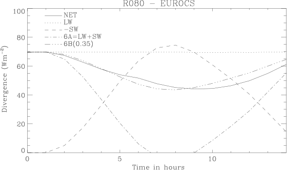
|
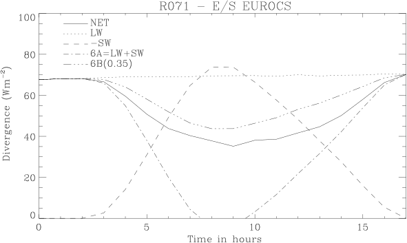
|
The 9C version attempted to remove the grid-dependence implied by the summation over 3 grid-levels in (468) as follows:
the search for the level with maximum LW radiative cooling, \(k_m\), is restricted to the top half of the mixed layer and no higher than level NTML\(+1\)
to allow for the case where the radiative cooling is distributed roughly equally over two grid-levels, if the LW flux divergence in level \(k_m-1\) is greater than half that in level \(k_m\), then \(k_m\) is lowered one grid-level.
then, the cloud-top radiative flux change is initially calculated for LW and SW fluxes separately as:
(471)#\[\Delta_F= F_{k_m+1} - F_{k_{rb}}\]where the base grid-level for the calculation, \(k_{rb}\), is taken to be the higher of the base of the LW radiatively cooled layer and \(z_h/2\), since cooling can only generate turbulence if it occurs in the upper part of the mixed layer. For decoupled stratocumulus layers, \(k_{rb}\) is further restricted to be above the top of the surface mixed layer.
finally, the flux divergence across grid-level \(k_m+1\) is separated into cloudy and free-atmospheric contributions by extrapolating the free-atmospheric flux-gradient downwards. The cloudy contribution is then included in \(\Delta F\):
(472)#\[\Delta F= \Delta F+ \Delta_{k_m+\frac{3}{2}} F - \Delta_{k_m+\frac{5}{2}} \frac{\Delta_{k_m+\frac{3}{2}} z}{k_m+\frac{1}{2}} F\]As at 9B above, the calculations in (471) and (472) are performed separately for LW and SW radiation before the two are combined using the empirical relationship in (470)
Further single column model tests with fine vertical resolution have shown the above calculations can still fail to accurately measure the radiative flux jump across the top of the cloud. The methodology now recommended is to identify where the LW radiative cooling profile transitions from free-tropospheric rates above the cloud to stronger rates within it. It entails only relatively minor changes to the first two steps of the algorithm above which become:
the search for the level with maximum LW radiative cooling, \(k_m\), is restricted to the top half of the mixed layer and below \(1.2 \, z_{\mathrm{h}}\) (rather than level NTML\(+1\) used above)
if the LW flux divergence in level \(k_m+1\) is relatively weak (less than double that in level \(k_m+2\)), we assume that level \(k_m+1\) is actually typical of the free-troposphere and that \(k_m\) must therefore be the inversion grid-level (despite having the strongest LW cooling). Hence we lower \(k_m\) by one so that it now marks the top of the mixed layer – note that LW cooling within the inversion grid-level will be included in step 4 above (which is unchanged)
These small changes were found sufficient to give a robust measure of \(\Delta F\) for grids varying down to 20m spacing where the radiative flux profile is well resolved.
Appendix: Derivation and definitions of the buoyancy parameters#
Buoyancy is measured by the virtual temperature
where \(c_v=(1/\epsilon) -1\) and \(\epsilon\) is the ratio of the molecular weights of water vapour and dry air (i.e., \(\epsilon = M_v/M_a \approx 0.62198\)). The buoyancy flux is then given by
Linearising gives
where the buoyancy parameters are given by
In saturated cloudy air (see, for example, Stage and Businger (1981)), the Clausius-Clapeyron equation can be used to calculate \(\overline{w'q_{\ell}'}\) (via \(q_{\ell}' = q_t' - q_s' = q_t' - \alpha_L T'\)) as
where
where R is the gas constant (\(=287.05\)). Thus the buoyancy flux can be written
where
Note that here \(\tilde{\beta_T}\) and \(\tilde{\beta_q}\) are strictly in-cloud parameters, while their definitions in boundary layer code prior to 8A were grid-box mean. Thus, here, any necessary \(C_F\)-weighting must be included explicitly, as in (217).
In all the above, if \(T\) is less than the melting point of ice then the latent heat of sublimation, \(L_s = L + L_f\), is used in place of \(L\).
Appendix: changing between specific humidities and mixing ratios#
Denote wet density by
where \(\rho_y\) is the density of dry air and the other \(\rho\) are vapour, liquid and frozen water respectively. Mixing ratios and specific humidities are then defined as
When specific quantities are mixed, the turbulent diffusion equations, (207) and (208), have \(\rho\) as the wet density. This is then consistent with the conservation of globally integrated quantities such as moisture. For example, neglecting spherical geometry for simplicity:
When mixing ratios are used, the momentum equations, (208), remain unchanged and the wet density still appears. This makes the reasonable assumption that all moisture components should be included in the momentum budget. For moisture conservation, (474) can be rewritten in terms of mixing ratios as
Thus \(\rho\) in (207) is replaced with \(\rho_y\) for \(\chi = m_t\) and \(\theta_{\ell}\) when mixing ratios are passed into the boundary layer code.
For surface exchange, JULES initially approximates the surface air density as \(\rho_* = p_S/(R T_S)\) (where the subscript \(S\) denotes the surface values and \(R\) the gas constant for dry air, 287 JK\(^{-1}\)kg\(^{-1}\)). If a more accurate calculation of surface air density is requested, following Eqs (1) to (6) of Webb et al. (1980) we then calculate the wet or dry surface air densities (to be used when the atmospheric humidity is specific or mixing ratio, respectively) as:
where, in each case, the surface humidity is taken as the surface saturated humidity over open sea but over land and ice surfaces this is likely to be inappropriate and so the driving level humidity is used (typically the lowest model level).
Note that \(\theta_{\ell}\) itself is defined in terms of mixing ratios as:
For saturation calculations a version of QSAT is used that is switchable between input specific and mixing ratio variables. The rate of change of \(q_s\) with temperature is also used in the boundary layer code (see e.g. appendix Appendix: Derivation and definitions of the buoyancy parameters):
In fact this expression should really be converted to work for specific quantities and so simply changing to mixing ratios will improve the accuracy of this calculation.
Finally, in appendix Appendix: Derivation and definitions of the buoyancy parameters virtual temperature is defined in terms of specific variables as
In terms of mixing ratios this becomes
Linearising, however, gives
Thus, the same level of approximation as is currently used is maintained simply by changing specific variables to mixing ratios.
Additional points to note are:
the diagnostic of screen humidity, \(q\)1.5m, will remain as a specific humidity. Similarly RH1.5m will remain defined in terms of specific quantities, i.e., \(q\)1.5m\(/q_s\)1.5m
all other moisture diagnostics (e.g., latent heat fluxes and increments) will simply switch to being mixing ratios if mixing ratios are selected - no conversion will be made.
it is important to note that RHOKM will be wet density times \(K_m\) while RHOKH will be dry density times \(K_h\)
Appendix: including the heating from turbulence dissipation#
An estimate of the true molecular dissipation rate, \(\epsilon_{mol}\), can be obtained by assuming local equilibrium in the budget of subgrid TKE (SKE). Then the sum of the inputs from resolved kinetic energy, plus that from subgrid buoyancy effects, must equal the dissipation. The SKE budget is
where the shear production, S, is essentially the resolved KE dissipation term. Note that the buoyancy term B appears in (476) which indicates that some of the energy from resolved scale dissipation (i.e. S) should be consumed in doing work against buoyancy (at least in stable BLs) thus leaving less energy to be finally dissipated as heat. Note though that CBLs will generate additional dissipation (and hence heating) through the buoyancy term. Note that from an atmospheric budget viewpoint the transport term, T, can be neglected as it will integrate vertically to zero. Locally, vertical variations could be important but it will be ignored because finally the heating source is implemented through an integral over the BL.
So, this estimate of the molecular dissipation rate should appear as an additional heating source term, (following Zhang and Altshuler (1999)):
Tests in the SCM showed the heating rate gradients can be very large near the surface. Hence to avoid stability problems (since this heating increment must be added after the implicit calculation of the stress (and heat flux) profiles) the increments are summed over the levels within the BL (i.e. up to \(z_{\mathrm{h}}\) ) and then that total heating is applied as a linear decrease from the surface to zero over \(z_{\mathrm{h}}\) .
Appendix: Operational modifications#
The operational global forecast model has been found to give improved performance on NWP Index parameters when the following modifications to its local \(Ri\)-based scheme are used. In (226), the definition of \(\lambda_m\) only is altered to
and both \(\lambda_m\) and \(\lambda_h\) are not reduced (to 40m) above the boundary layer top. It is possible these modifications point to problems with the definition of the boundary layer depth and the use of a Prandtl number of unity with no stability dependence in the local scheme. Both these issues are under further investigation.
Appendix: Inputs to UKCA#
The UKCA chemistry and aerosols sub-model takes a number of boundary layer diagnostics as input. For a list of these and a brief explanation of how they are used see the table below. If any changes modify the results for these variables it will prevent UKCA jobs from regressing. If the changes are significant it would be prudent to discuss them with the UKCA code owner before lodging the change.
Boundary layer inputs to UKCA |
|||
Sec |
Item |
Description |
Use in UKCA |
0 |
24 |
SURFACE TEMPERATURE AFTER TIMESTEP |
dry deposition |
0 |
25 |
BOUNDARY LAYER DEPTH AFTER TIMESTEP |
dry deposition, bl nucleation and call to tr_mix |
0 |
26 |
ROUGHNESS LENGTH AFTER TIMESTEP |
dry deposition |
0 |
233 |
SURFACE TEMPERATURE ON TILES K |
dry deposition |
0 |
234 |
ROUGHNESS LENGTH ON TILES m |
dry deposition |
3 |
60 |
RHOKH_MIX |
call to tr_mix |
3 |
64 |
D TRDZ_CHARNEY_GRID |
call to tr_mix |
3 |
65 |
GRID-LEVEL OF SML INVERSION (kent) |
call to tr_mix |
3 |
66 |
Rho * entrainment rate (we_lim) |
call to tr_mix |
3 |
67 |
Fraction of the timestep (t_frac) |
call to tr_mix |
3 |
68 |
zrzi |
call to tr_mix |
3 |
69 |
GRID-LEVEL OF DSC INVERSION (kent) |
call to tr_mix |
3 |
70 |
Rho * entrainment rate dsc |
call to tr_mix |
3 |
71 |
Fraction of the timestep dsc |
call to tr_mix |
3 |
72 |
zrzi dsc |
call to tr_mix |
3 |
73 |
ZHSC Top of decoupled layer |
call to tr_mix |
3 |
217 |
SURFACE HEAT FLUX W/M2 |
dry deposition |
3 |
230 |
10 METRE WIND SPEED ON C-GRID |
calculate sea salt emissions |
3 |
401 |
Dust Emissions div 1 |
GLOMAP dust scheme |
3 |
402 |
Dust Emissions div 2 |
GLOMAP dust scheme |
3 |
403 |
Dust Emissions div 3 |
GLOMAP dust scheme |
3 |
404 |
Dust Emissions div 4 |
GLOMAP dust scheme |
3 |
405 |
Dust Emissions div 5 |
GLOMAP dust scheme |
3 |
406 |
Dust Emissions div 6 |
GLOMAP dust scheme |
3 |
430 |
Dust Friction velocity (U*) on tiles |
dry deposition |
3 |
462 |
STOMATAL CONDUCTANCE ON PFTS (M/S) |
dry deposition |
3 |
465 |
FRICTION VELOCITY |
dry deposition |
3 |
473 |
TURBULENT KINETIC ENERGY |
ACTIVATE cloud scheme |
Appendix: Notation#
Finite difference notation |
|
\(z_k\) |
height of the \(\theta\)-level \(k\) |
\(z_{k+\frac{1}{2}}\) |
height of half-level above \(\theta\)-level \(k\) |
\(\Delta_k\) |
indicates a finite difference between \(\theta\)-levels \(k\) and \(k-1\) |
\(\Delta_{k+\frac{1}{2}}\) |
indicates a finite difference between half-levels \(k+\frac{1}{2}\) and \(k-\frac{1}{2}\) |
\(\Delta\) |
note: real change (i.e., not necessarily finite-difference) in a parameter |
across the capping inversion (see (467) and following text) |
Model variables |
|
\(\theta_l\), \(\theta_{v\ell}\) |
|
\(T_v\), \(\theta_v\) |
virtual temperature and potential temperature, |
defined by (473) and in section (Calculation of parcel buoyancy excess) |
|
\(b\) |
buoyancy (\(=g T_v'/T_v\)) |
\(q_t\), \(q_v\), \(q_s\), \(q_{\ell}\), \(q_f\) |
specific humidities: |
total, vapour, saturated, liquid and frozen water, respectively |
|
\(C_F\), \(C_F^l\), \(C_F^f\) |
cloud fraction and the liquid and frozen water parts, respectively |
\({\mathcal{H}}\) |
total heat flux (net radiative plus turbulent, Kms\(^{-1}\)) |
Thresholds |
|
\(C_t\) |
(\(=1.1\)) threshold for ratio of layer \(q_t\)-gradients in cumulus diagnosis |
\(\Gamma_{\mathrm{inv}}\) |
(\(=1.1\)) threshold on ratio of environment to parcel \(\theta_v\) gradients |
for identifying capping inversions above the LCL |
|
SC_CFTOL |
(\(=0.1\)) \(C_F\) threshold for recognising the presence of Sc |
\(\Delta_{k_{ct}} \theta_{v\ell}/ \Delta_{k_{ct}} z < 10^{-3}\) |
threshold (in Km\(^{-1}\)) for initial diagnosis of well-mixed DSC layers |
\(D_t\) |
(\(=0.1\)) threshold for the ratio of buoyancy consumption to production |
before decoupling occurs |
Layer definitions and parameters |
|
SML |
surface-based mixed layer |
NTML |
top \(\theta\)-level within SML |
NTPAR |
top \(\theta\)-level reached by parcel ascent |
DSC |
decoupled stratocumulus (mixed layer) |
NTDSC |
top \(\theta\)-level within DSC layer |
NBDSC |
bottom \(\theta\)-level within DSC layer |
NTLOC |
top \(\theta\)-level below which \(Ri<1\) |
\(z_{\mathrm{h}}\) |
height of top of SML (potentially subgrid) |
\(z_{\mathrm{h}}^{\mathrm{Sc}}\) |
height of top of DSC layer (potentially subgrid) |
\(z_{\mathrm{b}}\) |
height of base of DSC layer (subgrid) |
\(z_{\mathrm{par}}\) |
height of half-level at top of parcel ascent |
\(z_{\mathrm{loc}}\) |
height of half-level marking ‘top’ of local \(Ri\)-based mixing |
(where \(Ri>1\)) |
|
\(z_i\) |
generic inversion height |
\(z_c\) |
cloud depth |
\(z_{\mathrm{ml}}\) |
mixed layer depth |
\(K_m^{\mathrm{surf}}\), \(K_h^{\mathrm{surf}}\) |
\(K\) profiles for surface-driven turbulence (in SML) |
\(K_m^{\mathrm{Sc}}\), \(K_h^{\mathrm{Sc}}\) |
\(K\) profiles for cloud-top-driven turbulence |
(calculated for both DSC and SML) |
|
LCL |
lifting condensation level |
Other parameters |
|
\(\gamma_{\theta_{\ell}}\) |
gradient adjustment term, given by (239) |
\(w_m\) |
scaling velocity for momentum mixing in the SML |
(used in \(K_m^{\mathrm{surf}}\), \(\gamma_{\theta_{\ell}}\) and the SML parcel perturbation, \(\theta_v'\)) |
|
\(w_*\) |
‘standard’ convective velocity scale for a cloud-free convective |
boundary layer, \(w_*^3 = z_{\mathrm{h}}\overline{w'b}_S\) |
|
\(u_*\) |
friction velocity (here includes the orographic component) |
\(w_e\), \(\tilde{w_e}\) |
entrainment velocity and compensated to allow for subsidence (ms\(^{-1}\)) |
\(w_S\) |
subsidence velocity (ms\(^{-1}\)) |
\(\Delta_F\) |
cloud-top net radiative divergence, calculation given in (468) |
\(\alpha_t\) |
parameter in entrainment parametrization, (247) |
\(\tau_{rc}\), \(z_{rc}\) |
parameters in perturbation calculation, (216), |
for initial identification of and \(z_{\mathrm{ml}}\) calculation for DSC layers |
|
\(a_L\), \(\alpha_L\), \(\beta_T\), \(\beta_q\), \(\tilde{\beta_T}\), \(\tilde{\beta_q}\) |
buoyancy parameters, defined in appendix Appendix: Derivation and definitions of the buoyancy parameters |
References#
A. P. Lock and A. R. Brown and M. R. Bush and G. M. Martin and R. N. B. Smith (2000). A New Boundary Layer Mixing Scheme. Part I: Scheme Description and Single-Column Model Tests. Mon. Wea. Rev., 128, 3187-3199.
A. P. Lock and A. R. Brown and M. R. Bush and G. M. Martin and R. N. B. Smith (2001). Corrigendum. Mon. Wea. Rev., 129, 905-905.
G. M. Martin and M. R. Bush and A. R. Brown and A. P. Lock and R. N. B. Smith (2000). A New Boundary Layer Mixing Scheme. Part II: Tests in Climate and Mesoscale Models. Mon. Wea. Rev., 128, 3200-3217.
A. P. Lock (2001). The Numerical Representation of Entrainment in Parametrizations of Boundary Layer Turbulent Mixing. Mon. Wea. Rev., 129, 1148-1163.
A. R. Brown and A. L. M. Grant (1997). Non-local mixing of momentum in the convective boundary layer. Bound.-Layer Meteor., 84, 1-22.
N. Wood and A. R. Brown and F. E. Hewer (2001). Parametrizing the effects of orography on the boundary layer: An alternative to effective roughness lengths. Quart. J. Roy. Meteor. Soc., 127, 759-777.
A. R. Brown and R. J. Beare and J. M. Edwards and A. P. Lock and S. J. Keogh and S. F. Milton and D. N. Walters (2008). Upgrades to the Boundary-Layer Scheme in the Met Office Numerical Weather Prediction Model. Bound.-Layer Meteor., 128, 117-132.
I B Troen and L. Mahrt (1986). A simple model of the atmospheric boundary layer; sensitivity to surface evaporation. Bound.-Layer Meteor., 37, 129-148.
R. N. B. Smith (1990). A scheme for predicting layer clouds and their water content in a general circulation model. Quart. J. Roy. Meteor. Soc., 116, 435-460.
A. A. M. Holtslag and C.-H. Moeng (1991). Eddy Diffusivity and Countergradient Transport in the Convective Atmospheric Boundary Layer. J. Atmos. Sci., 48, 1690-1698.
A. P. Lock (1998). The parametrization of entrainment in cloudy boundary layers. Quart. J. Roy. Meteor. Soc., 124, 2729-2753.
A. P. Lock and M. K. Macvean (1999). The parametrization of entrainment driven by surface heating and cloud-top cooling. Quart. J. Roy. Meteor. Soc., 125, 271-299.
H.A. Panofsky and H. Tennekes and D.H. Lenschow and J.C. Wyngaard (1977). The characteristics of turbulent velocity components in the surface layer under convective conditions. Bound.-Layer Meteor., 11, 355-361.
A. C. M. Beljaars (1987). The influence of sampling and filtering on measured wind gusts. J. Atmos. Ocean. Techn., 4, 613-626.
A.C.M. Beljaars and A.A.M. Holtslag (1991). Flux Parametrization over Land Surfaces for Atmospheric Models. J. Appl. Meteor., 30, 327-341.
N. Wood and P. Mason (1993). The Pressure force induced by neutral, turbulent flow over hills. Quart. J. Roy. Meteor. Soc., 119, 1233-1267.
A. P. Lock (2009). Factors influencing cloud area at the capping inversion for shallow cumulus clouds. Quart. J. Roy. Meteor. Soc., 135, 941-952.
J.-L. Redelsperger and F. Guichard and S. Mondon (2000). A Parametrization of Mesoscale Enhancement of Surface Fluxes for Large-Scale Models. J. Climate, 13, 402-421.
A. A. M. Holtslag and B. A. Boville (1993). Local Versus Nonlocal Boundary-Layer Diffusion in a Global Climate Model. J. Climate, 6, 1825-1842.
Ayra, S. P. (1991). Finite-Difference Errors in Estimating of Gradients in the Atmospheric Surface Layer. J. Appl. Meteor., 30, 251-253.
Bodas-Salcedo, A. and K. D. Williams and P. R. Field and A. P. Lock (2012). Contribution of midlatitude cyclone clouds to the short-wave deficit in the Southern Ocean. J. Climate, 25, 7467-7486.
Bolton, D. (1980). The Computation of Equivalent Potential Temperature. Mon. Wea. Rev., 108, 1046-1053.
Brown, A. R. (1996). Large-eddy simulation and parametrization of the baroclinic boundary-layer. Quart. J. Roy. Meteor. Soc., 122, 1779-1798.
Brown, A. R. (1999). The sensitivity of large-eddy simulations of shallow cumulus convection to resolution and sub-grid model. Quart. J. Roy. Meteor. Soc., 125, 469-482.
Brown, A. R. and A. C. M. Beljaars and H. Hersbach (2006). Errors in parametrizations of convective boundary layer turbulent momentum mixing. Quart. J. Roy. Meteor. Soc., 132, 1859-1876.
Bush, M. R. and A. P. Lock and R. N. B. Smith (1999). Testing of the new boundary layer scheme in the Mesoscale Model. NWP Tech Report, 260.
Cullen, M. J. P. and J. A. James (1994). A comparison of two vertical grid staggerings. FR Sci Paper, 27.
Derbyshire, S. H. (1997). Recommendations for UM parametrization of stable boundary layers. Cardington Tech Note, 38.
Driedonks, A. G. M. (1982). Models and observations of the growth of the atmospheric boundary layer. Bound.-Layer Meteor., 23, 283-306.
Dyer, A. J. (1974). A review of flux-profile relationships. Bound.-Layer Meteor., 7, 363-372.
Edwards, J. M. (2007). Oceanic Latent Heat Fluxes: Consistency with the atmospheric hydrological and energy cycles and general circulation modeling. J. Geophys. Res., 112, D06115.
Essery, R. and Best, M. and Cox, P (2001). Moses 2.2 technical documentation. Hadley Centre Technical Note, 30.
Godfrey, J. S. and Beljaars, A. C. M. (1991). On the turbulent fluxes of buoyancy, heat and moisture at the air-sea interface at low wind speeds. J. Geophys. Res., 96, 22043-22048.
Hewer, F. E. and Wood, N. (1998). The effective roughness length for scalar transfer in neutral conditions over hilly terrain. Quart. J. Roy. Meteor. Soc., 124, 659-685.
Lock, A. P. (1999). A parametrization of turbulent mixing in convective cloud-capped boundary layers derived from large-eddy simulations. Proceedings of GCSS-WGNE Workshop on ‘Cloud processes and cloud feedbacks in large-scale models’, 9-13 November 1998, ECMWF, Shinfield Park, Reading, Berks., RG2 9AX, U.K..
Lock, A. P. (2012). Stable boundary layer modelling at the Met Office. ECMWF Workshop on Diurnal Cycles and the Stable Boundary Layer, 137-148.
Louis, J.-F. (1979). A parametric model of vertical eddy fluxes in the atmosphere. Bound.-Layer Meteor., 17, 187-202.
Mahrt, L. (1976). Mixed layer moisture structure. Mon. Wea. Rev., 104, 1403-1407.
Mason, P. J. (1986). On the parametrization of orographic drag. ECMWF Seminar on Physical Parametrization for Numerical Models of the Atmosphere, 2, 139-165.
Nicholls, S. and J. D. Turton (1986). An observational study of the structure of stratiform cloud sheets. Part II: Entrainment. Quart. J. Roy. Meteor. Soc., 112, 461-480.
Smith, S. D. (1988). Coefficients for sea surface wind stress, heat flux and wind profiles as a function of wind speed and temperature. J. Geophys. Res., 93, 15467-15472.
Stage, S. A. and J. A. Businger (1981). A model for entrainment into a cloud-topped marine boundary layer. Part I: Model description and application to a cold-air outbreak episode. J. Atmos. Sci., 38, 2213-2229.
Turton, J. D. and S. Nicholls (1987). A study of the diurnal variation of stratocumulus using a multiple mixed layer model. Quart. J. Roy. Meteor. Soc., 113, 969-1009.
Webb, E.K. and Pearman, G.I. and Leuning, R. (1980). Correction of flux measurements for density effects due to hear and water vapour transfer. Quart. J. Roy. Meteor. Soc., 106, 85-100.
Wood, N. and Diamantakis, M. and Staniforth, A. (2007). A monotonically-damping second-order-accurate unconditionally-stable numerical scheme for diffusion. Quart. J. Roy. Meteor. Soc., 133, 1559-1573.
Zhang, D.-L. and Altshuler, E. (1999). The effects of dissipative heating on hurricane intensity. Mon. Wea. Rev., 127, 3032-3038.
Zilitinkevich, S. S. (1975). Comments on ‘’A model for the dynamics of the inversion above a convective boundary layer’’. J. Atmos. Sci., 32, 991-992.
Siems, S. T. and Bretherton, C. S. and Baker, M. B. and Shy, S. and Breidenthal, R. E. (1990). Buoyancy reversal and cloud-top entrainment instability. Quart. J. Roy. Meteor. Soc., 116, 705-739.
Mailhot, J. and Lock, A. P. (2004). An examination of several parametrizations of mixing lengths in a stable boundary layer: the GABLS case.
Honnert, R. and Masson, V. and Couvreux, F. (2011). A Diagnostic for Evaluating the Representation of Turbulence in Atmospheric Models at the Kilometric Scale. J. Atmos. Sci., 68, 3112-3131. https://doi.org/10.1175/JAS-D-11-061.1
Malavelle, F. F. and Haywood, J. M. and Field, P. R. and Hill, A. A. and Abel, S. J. and Lock, A. P. and Shipway, B. J. and McBeath, K. (2014). A method to represent sub-grid scale updraft velocity in km-scale models: implication for aerosol activation. J. Geophys. Res., 119, 4149-4173. https://doi.org/10.1002/2013JD021218
Boutle, I. A. and Eyre, J. E. J. and Lock, A. P. (2014). Seamless stratocumulus simulation across the turbulent gray zone. Mon. Wea. Rev., 142, 1655-1668. https://doi.org/10.1175/MWR-D-13-00229.1
Beare, R. J. (2008). The role of shear in the morning transition boundary layer. Bound.-Layer Meteor., 129, 395-410.
Suselj, K. and Teixeira, J. and Matheou, G. (2012). Eddy Diffusivity/Mass Flux and Shallow Cumulus Boundary Layer: An Updraft PDF Multiple Mass Flux Scheme. J. Atmos. Sci., 69, 1513-1533.
G. T. Csanady (2001). Air-sea interaction: Laws and Mechanisms.
C. W. Fairall and E. F. Bradley and J. E. Hare and A. A. Grachev and J. B. Edson (2003). Bulk parametrization of air-sea fluxes: Updates and Verification for the COARE Algorithm. J. Climate, 16, 571-591.
J. B. Edson and V. Jampana and R. A. Weller and S. P. Biggore and A. J. Plueddemann and C. W. Fairall and S. D. Miller and L. Mahrt and D. VIckers and H. Hersbach (2013). On the exchange of momentum over the open ocean. J. Phys. Oceanogr., 43, 1589-1610.
R. Atlas and R. N. Hoffman and J. Ardizzone and S. M. Leidner and J. C. Jusem and D. K. Smith and D. Gombos (2011). A cross-calibrated, multiplatform ocean surface wind velocity product for meteorological and oceanographic applications. Bull. Amer. Meteorol. Soc., 92, 157-174, doi:10.1175/2010BAMS2946.1.
E. L. Andreas and T. W. Horst and A. A. Grachev and P. O. G. Persson and C. W. Fairall and P. S. Guest and R. E. Jordan (2010). Parametrizing turbulent exchange over summer sea ice and the marginal ice zone. Q. J. R. Meteorol. Soc., 136, 927-943.
C. Lupkes and V. M. Gryanik and J. Hartmann and E. L. Andreas (2012). A parametrization, based on sea ice morphology of the neutral atmospheric drag coefficients for weather prediction and climate models. J. Geophys. Res., 117, D13112. https://doi.org/10.1029/2012JD017630
C. Lupkes and V. M. Gryanik (2015). A stability-dependent parametrization of transfer coefficients for momentum and heat over polar sea to be used in climate models. J. Geophys. Res. Atmos., 120, 552-581. https://doi.org/10.1002/2014JD022418
A. D. Elvidge and I. A. Renfrew and A. I. Weiss and I. M. Brooks and T. A. Lachlan-Cope and J. C. King (2016). Observations of surface momentum exchange over the marginal ice zone and recommendations for irs parametrisation. Atmos. Chem. Phys., 16, 1545-1563. https://doi.org/10.5194/acp-16-1545-2016
D. Schroder and T. Vihma and A. Kerber and B. Brummer (2003). On the parameterization of turbulent surface fluxes over heterogeneous sea ice surfaces. J. Geophys. Res., 108(C6), 3195. https://doi.org/10.1029/2002JC001385
M. A. Donelan and B. K. Haus and N. Reul and W. J. Plant and M. Sriassnie and H. C. Graber and O. B. Brown and E. S. Saltzman (2004). On the limiting aerodynamic roughness of the ocean in very strong winds. Geophys. Res. Lett., 31, L18306. https://doi.org/10.1029/2004GL019460
Donelan, M. A. (2018). On the decrease of the oceanic drag coefficient in high winds. J. Geophys. Res: Oceans, 123, 1-17. https://doi.org/10.1002/2017JC013394
Hsu, J. and Lien, R. and D’Asaro, E. A. and Sanford, T. B. (2017). Estimates of Surface Wind Stress and Drag Coefficients in Typhoon Megi. J. Phys. Oceanogr., 47, 545-565. https://doi.org/10.1175/JPO-D-16-0069.1