Filtering by Convolution

The convolution method (see Convolution) applies a scale-selective filter \(\mathcal{L}\) to the difference between the model field and the reference field, so that only the large scales are nudged. This section explains why the filter is applied as a convolution in physical space, and derives the convolution kernel used on the sphere.

Consider filtering a field \(f\) so that only its large scales are retained. Writing the spectrum of \(f\) as \(\mathcal{F}[f]\), where \(\mathcal{F}\) denotes a transform to spectral space, the filter \(\mathcal{L}\) acts as a multiplication of the spectrum by a function \(\ell\) that varies with wavenumber:

(211)\[\mathcal{L}[f] = \mathcal{F}^{-1}\left[ \ell \; \mathcal{F}[f] \right] .\]

It is vital that \(\ell\) does not amplify any wavenumbers, which will cause the numerical model to go unstable. However, it is not always necessary for an analytic form of \(\ell\) to be preserved exactly by the discretisation. For example, an idealised “top-hat” may be specified for \(\ell\), but it may be acceptable for the discretisation to only approximate this.

Why a convolution?

The most direct way to apply (211) would be to transform \(f\) to spectral space, multiply by \(\ell\), and transform back. However, for a parallel implementation in which \(f\) is distributed geographically across many processors, this is very inefficient: the transform requires global gather and scatter communications and/or global summations, whose cost grows exponentially with the number of processors.

An alternative is to note the convolution theorem: the spectrum of a convolved field is the product of the spectra of the field and of the convolving function. Defining the convolution of \(f\) with a function \(c\) as

(212)\[\mathcal{C}[f, c] := \int_\Omega f(\boldsymbol{y}) \; c(\boldsymbol{y} - \boldsymbol{x}) \; \mathrm{d}\boldsymbol{y} \equiv f \ast c ,\]

the convolution theorem gives \(\mathcal{F}\!\left[\mathcal{C}[f, c]\right] = \mathcal{F}[f] \, \mathcal{F}[c]\). Since the filter (211) acts as a multiplication in spectral space, it can therefore be applied as a convolution in physical space, provided the convolving function is chosen so that \(\mathcal{F}[c] = \ell\), i.e. \(c = \mathcal{F}^{-1}[\ell]\).

The key advantage is that, if \(c\) has compact support, the integral in (212) reduces to an integral over a local neighbourhood of each point. On a distributed mesh this requires only communication of neighbouring data through halo exchanges, rather than the global communications demanded by a spectral transform.

In practice the convolution is truncated by restricting it to a local stencil of finite extent. The truncated kernel is no longer exactly equal to \(\mathcal{F}^{-1}[\ell]\), but can remain a good approximation provided the truncation occurs where \(c\) is already small. When the nudging of the spectrum does not need to be exact, this can be acceptable.

The filter on the sphere

To apply this approach on the cubed-sphere, the convolution kernel must be derived for the sphere. The cubed-sphere is non-orthogonal and has discontinuities at panel edges, which makes a separable longitude–latitude Fourier filter challenging. Instead, the field is expanded in spherical harmonics, which are appropriate for quasi-uniform meshes of the sphere. This use of a convolution for scale-selective filtering on a cubed-sphere follows the approach of Thatcher and McGregor (2009).

The spherical harmonics, as functions of co-latitude \(\theta\) and longitude \(\varphi\), may be written as

(213)\[Y_{lm}(\theta, \varphi) = N_{lm} \, e^{i m \varphi} \, P_{lm}(\cos\theta) ,\]

where \(P_{lm}\) are the associated Legendre polynomials and \(N_{lm}\) is a normalisation chosen so that the \(Y_{lm}\) are orthonormal over the sphere. A field \(f\) is expanded as \(f(\theta,\varphi) = \sum_{l,m} a_{lm} Y_{lm}(\theta,\varphi)\).

We seek the convolution kernel \(c\) that retains only the spherical harmonic components with total wavenumber between \(k_{min}\) and \(k_{max}\). Since the spherical harmonics form an orthonormal basis, this filter kernel can be written

(214)\[c(\theta,\varphi,\theta',\varphi') = \sum_{l=k_{min}}^{k_{max}} \sum_{m=-l}^{l} F_{lm} \, Y_{lm}(\theta,\varphi) \, Y_{lm}^{\ast}(\theta',\varphi') .\]

The kernel should depend only on the distance between two points, and not on their orientation. This requires that there is no dependence on \(m\) or \(\varphi\), so that \(F_{lm} = F_{l0}\). The sum over \(m\) can then be carried out using the spherical harmonic addition theorem,

(215)\[\sum_{m=-l}^{l} Y_{lm}(\theta,\varphi) \, Y_{lm}^{\ast}(\theta',\varphi') = \frac{2l+1}{4\pi} \, P_l\!\left(\cos\gamma\right) ,\]

where \(P_l\) is the Legendre polynomial of degree \(l\) and \(\gamma\) is the great-circle (central) angle between the two points. Taking an idealised top-hat filter in spectral space, \(F_{l0} = 1\), the kernel becomes a weighted sum of Legendre polynomials of the central angle:

(216)\[c(\gamma) = \sum_{l=k_{min}}^{k_{max}} \frac{2l+1}{4\pi} \, P_l(\cos\gamma) .\]

The Legendre polynomials may be evaluated efficiently using the recurrence relation

(217)\[\begin{split}\begin{aligned} P_0(\cos\gamma) &= 1 , \\ P_1(\cos\gamma) &= \cos\gamma , \\ P_l(\cos\gamma) &= \frac{2l-1}{l} \cos\gamma \, P_{l-1}(\cos\gamma) - \frac{l-1}{l} \, P_{l-2}(\cos\gamma) . \end{aligned}\end{split}\]

Equation (216) is the kernel that corresponds exactly to the idealised top-hat spectral filter. It resembles a \(\mathrm{sinc}\) function, (mainly!) decaying away from \(\gamma = 0\), and is evaluated at the points of the stencil surrounding each grid point to give the discrete convolution weights.

Convolution Envelope

However the series of Legendre polynomials does not strictly have compact support and extends over the whole sphere. An accurate convolution would therefore require a stencil covering the whole domain.

Instead we truncate the filter to a local stencil. To avoid the spurious amplification of any wavenumbers, the filter is multiplied by a Gaussian envelope that decays to zero towards the edge of the stencil. The width of this envelope is a configurable parameter of the scheme, and must be chosen together with the stencil extent (see Nudging for guidance).

Thus the actual filter used is

(218)\[c(\gamma) = \left[ \sum_{l=k_{min}}^{k_{max}} \frac{2l+1}{4\pi} P_l(\cos\gamma) \right] \exp\left[ -\frac{1}{2} \left( \frac{\gamma}{\sigma} \right)^2 \right] ,\]

where \(\gamma\) is the great-circle angle from the central point and \(\sigma\) is the width of the Gaussian envelope.

Fig. 4 illustrates the effect of the envelope. The underlying Legendre filter (216) oscillates and decays only slowly with distance, so that it does not have compact support. Multiplying by the Gaussian envelope gives the enveloped filter, which decays smoothly to zero well within the stencil, allowing the convolution to be truncated to a local region with minimal error, provided the stencil is wide enough for the envelope to have decayed sufficiently by its edge.

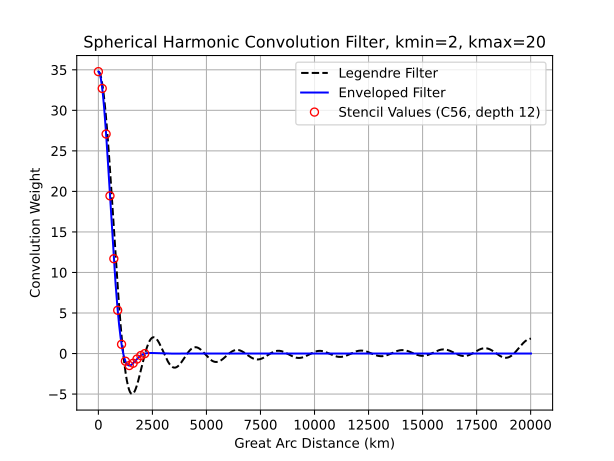
Fig. 4 The spherical-harmonic convolution filter for a top-hat retaining total wavenumbers from \(k_{min} = 2\) to \(k_{max} = 20\), plotted against great-circle distance. The underlying Legendre filter (black dashed, (216)) oscillates and decays only slowly, whereas the enveloped filter (blue, (218)) decays smoothly to zero. The red circles show the discrete filter values sampled at the stencil points for a stencil of depth 12 on a C56 mesh.