


Setting up the environment#
The first step is to set up the conda environment. You should use the profsea-env.yml environment file, building it with
conda env create -f profsea-env.yml
and then activating with conda activate profsea.
One final step here is to install ProFSea as an editable package, using
pip install -e .
while inside the highest level directory.
Importing components#
The next step is to import all the model components you want to run simulations with - a full list is available in the documention here. This can be any combination of available global and spatial components, how you build your model is up to you!
To generate a comprehensive set of sea-level projections, we’ll run with all the components that contribute to sea-level change:
thermal expansion
glaciers
greenland ice-sheet
antarctic ice-sheet
landwater
In the example below, we’ll run with the configuration being used for SLEIP and Munday et al. (2026), in prep.
[12]:
from profsea.components.core.global_model import Global
from profsea.components.global_ import (
    AntarcticaISMIP6,
    Glacier,
    GreenlandAR6,
    LandwaterAR6,
    ThermalExpansion,
)
ProFSea can run with a single or an ensemble of temperature and ocean heat content forcing trajectories. The trajectories need to be anomalies, relative to some baseline reference period, which we assume in this notebook is 1986-2005.
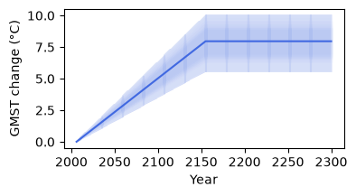
Here we’ll just run with an idealised temperature ramp up and stabilisation, and corresponding ocean heat content change, running from 2006 to 2300:
[13]:
import matplotlib.pyplot as plt
import numpy as np

t_change = np.concatenate([np.linspace(0.01, 8, 150), np.linspace(8, 8, 145)])
t_change = t_change[None, :] * np.random.normal(
    loc=1.0, scale=0.1, size=(100, 1)
)  # add some variability across members
ohc_change = t_change * 1e24  # in Joules
years = np.arange(2006, 2301)
years = np.broadcast_to(years, t_change.shape)

plt.figure(figsize=(4, 2))
plt.plot(years, t_change, color="royalblue", alpha=0.1)
plt.plot(
    years.mean(axis=0), t_change.mean(axis=0), color="royalblue", label="GMST change"
)
plt.xlabel("Year")
plt.ylabel("GMST change (°C)")
plt.show()
plt.close()
Building the model#
To build your model, simply add your components to a dictionary, with whatever names you like, and pass it to the Global() class
[14]:
global_components = {
    "landwater": LandwaterAR6(),
    "greenland": GreenlandAR6(),
    "expansion": ThermalExpansion(
        ohc_change
    ),  # only the thermal expansion needs OHC change, so we'll pass it in here
    "wais": AntarcticaISMIP6(region="wais"),
    "eais": AntarcticaISMIP6(region="eais"),
    "peninsula": AntarcticaISMIP6(region="peninsula"),
    "glacier": Glacier(),
}
global_model = Global(
    components=global_components,
    start_yr=2006,
    end_yr=2301,
    baseline_start=1986,
    baseline_end=2005,
    num_members=1000
)
now we’re ready to run our simulation…
[15]:
projections = global_model.run(
    T_change=t_change, scenario="stabilisation", member_seed=42
)
global_model.sum_components(projections)
gmslr = global_model.results["total_gmslr"]
╭────────────────────────── Baseline Check ──────────────────────────╮
│ Check that all input data (GSAT, OHC, and zostoga) are provided    │
│ relative to the same reference period as given to ProFSea. If they │
│ use a different baseline, re-baseline them before calling run().   │
│                                                                    │
│  Baseline Start:  1986                                             │
│    Baseline End:  2005                                             │
╰────────────────────────────────────────────────────────────────────╯
╭──────────────────────── ProFSea Global Run Configuration ─────────────────────────╮
│        Scenario  stabilisation                                                    │
│      Components  landwater, greenland, expansion, wais, eais, peninsula, glacier  │
│        Baseline  1986 -> 2005                                                     │
│       Timeframe  2006 -> 2301                                                     │
│   Ensemble Size  100 inputs × 1000 draws (= 100000)                               │
│          Output  Full Distribution (100000 members)                               │
│  Compute Engine  Parallel Threading                                               │
╰───────────────────────────────────────────────────────────────────────────────────╯
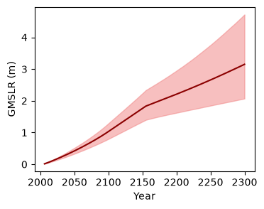
visualise the global simulations!
[16]:
plt.figure(figsize=(4, 3))
lower = np.percentile(gmslr, 5, axis=(0, 1))
upper = np.percentile(gmslr, 95, axis=(0, 1))
plt.fill_between(
    years[0], lower, upper, color="lightcoral", alpha=0.5, label="90% range"
)
plt.plot(years[0], gmslr.mean(axis=(0, 1)), color="darkred")
plt.xlabel("Year")
plt.ylabel("GMSLR (m)")
plt.show()
plt.close()
Building the Spatial model#
Start with the imports:
[17]:
from profsea.components.core import Spatial
from profsea.components.spatial import (
    GIA,
    Fingerprint,
    SterodynamicCMIP6,
)
Now we’ll build the model in the same way as the global model, but we’ll pass the individual components’ global projections to each spatial module.
[18]:
spatial_components = {
    "sterodynamic": SterodynamicCMIP6(
        projections["expansion"],  # passing in the global thermal expansion projection
    ),
    "greenland": Fingerprint(
        projections["greenland"], fingerprint_component="greenland"
    ),
    "landwater": Fingerprint(
        projections["landwater"],
        fingerprint_component="landwater",
    ),
    "wais": Fingerprint(
        projections["wais"],
        fingerprint_component="wais",
    ),
    "eais": Fingerprint(
        projections["eais"],
        fingerprint_component="eais",
    ),
    "glacier": Fingerprint(
        projections["glacier"],
        fingerprint_component="glacier",
    ),
    "gia": GIA(
        sample_spatial=False,
    ),
}

# Pass to the spatial model
spatial_model = Spatial(
    components=spatial_components,
    baseline_yrs=(1986, 2005),  # same baseline as the Global model
)
spatial_model.run(member_seed=42)

total_rsl = spatial_model.sum_components(spatial_model.results)
[09:55:27] INFO ✓ ProFSea assets found locally!
[09:55:28] INFO ✓ ProFSea assets found locally!
INFO ✓ ProFSea assets found locally!
INFO ✓ ProFSea assets found locally!
INFO ✓ ProFSea assets found locally!
INFO ✓ ProFSea assets found locally!
INFO ✓ ProFSea assets found locally!
INFO ✓ ProFSea assets found locally!
INFO Baseline period = 1995 to 2014
╭─────────────────────── ProFSea Spatial Run Configuration ────────────────────────╮
│        Components  sterodynamic, greenland, landwater, wais, eais, glacier, gia  │
│         Timeframe  2006 -> 2301                                                  │
│          Baseline  1995 - 2014                                                   │
│   Grid Resolution  180 × 360 cells                                               │
│            Output  Percentiles: [5, 17, 50, 83, 95]                              │
│  Est. Output Size  ~0.76 GB                                                      │
╰──────────────────────────────────────────────────────────────────────────────────╯
INFO Simulating 7 sea-level components: sterodynamic, greenland, landwater, wais, eais, glacier, gia
Saving the spatial projections is easy + quick using Zarr format:
[19]:
spatial_model.save_components(
    spatial_model.results, scenario_name="stabilisation", output_format="zarr"
)
[09:57:14] INFO ✓ Successfully saved Zarr: ./stabilisation_projection.zarr
INFO Output shape for 'sterodynamic' was (5, 295, 180, 360) (percentile, time, lat, lon)
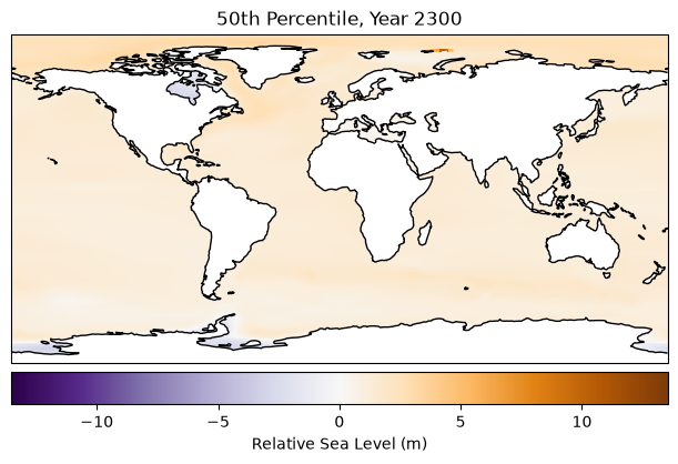
Plot the output! This takes about 90 seconds, since our data goes from lazy → in memory
[20]:
import cartopy.crs as ccrs

fig = plt.figure(figsize=(6, 4), layout="constrained")

total_rsl_med = total_rsl[2, -1, :, :]
vmax = np.nanmax(np.abs(total_rsl))
vmin = -vmax

ax = fig.add_subplot(111, projection=ccrs.PlateCarree())
ax.set_title("50th Percentile, Year 2300")
ax.pcolormesh(
    spatial_model.grid_lons,
    spatial_model.grid_lats,
    total_rsl_med,
    transform=ccrs.PlateCarree(),
    cmap="PuOr_r",
    vmin=vmin,
    vmax=vmax,
)
ax.coastlines()
fig.colorbar(
    mappable=ax.collections[0],
    label="Relative Sea Level (m)",
    orientation="horizontal",
    pad=0.02,
)
plt.show()
Next, we’ll drill down on a few grid-boxes of interest. To do this we can use the Local model.
We give the spatial components to our Local model, and a dictionary of locations with associated lat/lons:
[21]:
from profsea.components.core.local_model import Local

from profsea.components.core import Spatial
from profsea.components.spatial import (
    SterodynamicCMIP6,
    Fingerprint,
    GIA,
)

locations = {
    "Aberdeen": (57.144, -2.080),
    "Holyhead": (53.314, -4.620),
    "Llandudno": (53.330, -3.830),
    "Land point": (-34.6037, -58.3816),
}

local_components = {
    "sterodynamic": SterodynamicCMIP6(
        projections["expansion"],  # passing in the global thermal expansion projection
    ),
    "greenland": Fingerprint(
        projections["greenland"],
        fingerprint_component="greenland"
    ),
    "landwater": Fingerprint(
        projections["landwater"],
        fingerprint_component="landwater",
    ),
    "wais": Fingerprint(
        projections["wais"],
        fingerprint_component="wais",
    ),
    "eais": Fingerprint(
        projections["eais"],
        fingerprint_component="eais",
    ),
    "glacier": Fingerprint(
        projections["glacier"],
        fingerprint_component="glacier",
    ),
    "gia": GIA(
        sample_spatial=False,
    ),
}

local_model = Local(
    components=local_components,
    locations=locations,
    baseline_yrs=(1986, 2005),  # same baseline as the Global model
)
local_timeseries = local_model.run(member_seed=42)
total_rsl = local_model.sum_components(local_model.results)
[09:58:16] INFO ✓ ProFSea assets found locally!
INFO ✓ ProFSea assets found locally!
INFO ✓ ProFSea assets found locally!
INFO ✓ ProFSea assets found locally!
INFO ✓ ProFSea assets found locally!
INFO ✓ ProFSea assets found locally!
[09:58:17] INFO ✓ ProFSea assets found locally!
INFO ✓ ProFSea assets found locally!
INFO Baseline period = 1995 to 2014
INFO Configured for 4 specific target locations.
INFO Simulating 7 sea-level components for 4 sites...
[09:58:25] WARNING  The following site(s) may be over land: Land point. Expect NaN values for all components.
                    Either try increasing your grid resolution or check your site coordinates.
[22]:
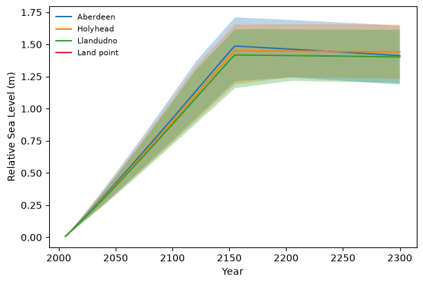
loc_ts = local_timeseries["total_rsl"].sel(site=["Aberdeen", "Holyhead", "Llandudno", "Land point"], percentile=[17, 50, 83])
fig = plt.figure(figsize=(6, 4), layout="constrained")
ax = fig.add_subplot(111)
for loc in loc_ts.site.values:
    loc_data = loc_ts.sel(site=loc)
    ax.fill_between(loc_data.time, loc_data.sel(percentile=17), loc_data.sel(percentile=83), alpha=0.3)
    ax.plot(loc_data.time, loc_data.sel(percentile=50), label=loc)
ax.set_xlabel("Year")
ax.set_ylabel("Relative Sea Level (m)")
ax.legend(frameon=False, loc="upper left", fontsize=8)

plt.show()