analysis module
Created on March, 2020 Authors: Dave Rowell, Grace Redmond, Saeed Sadri, Hamish Steptoe
-
analysis.calculate_dewpoint(P, Q, T)¶ A function to calculate the dew point temperature, it expects three iris cubes P, Q, T. Stash codes needed are 00001, 03237, 03236.
Parameters: - T (1.5m temperature cube) –
- Q (1.5m specific humidity cube) –
- P (P star cube) –
Returns: TD
Return type: 1.5m dew point temperature cube
Notes
Based on the UM routine /home/h04/precis/um/vn4.5/source/umpl/DEWPNT1A.dk which uses /home/h04/precis/um/vn4.5/source/umpl/QSAT2A.dk Constants:
- LC is the latent heat of condensation of water at 0 deg C.
- RL1 is the latent heat of evaporation
- TM is the temperature at which fresh waster freezes
- EPSILON is the ratio of molecular weights of water and dry air
- R the gas constant for dry air (J/kg/K)
- RV gas constant for moist air (J/kg/K)
This test compares dewpoint calculated by the calculate_dewpoint function, to dewpoint directly output from the UM i.e. uses the fortran routine
>>> file1 = os.path.join(config.DATA_DIR, 'dewpointtest_pt1.pp')
>>> file2 = os.path.join(config.DATA_DIR, 'dewpointtest_pt2.pp')
>>> P=iris.load_cube(file2, 'surface_air_pressure')
>>> T=iris.load_cube(file1, 'air_temperature')
>>> Q=iris.load_cube(file1, 'specific_humidity')
>>>
>>> DEWPOINT=iris.load_cube(file1, 'dew_point_temperature')
>>> TD = calculate_dewpoint(P, Q, T)
WARNING dewpoint temp. > air temp ---> setting TD = T
>>>
>>> diff = DEWPOINT - TD
>>> print(np.max(diff.data))
0.37731934
>>> print(np.min(diff.data))
-0.31027222
>>> print(np.mean(diff.data))
2.934921e-05
>>> print(np.std(diff.data))
0.0058857435
-
analysis.ci_interval(xi, yi, alpha=0.05)¶ Calculates Confidence interval (default 95%) parameters for two numpy arrays of dimension 1. Returns include the gradient and intercept of the confidence interval.
It also returns vectors for confidence interval plotting: - the high/low confidence interval of the slope - the high low curves of confidence interval of yi.
Parameters: - xi (numpy array of dimension 1) –
- yi (dependant variable, numpy array of dimension 1) –
- alpha (required confidence interval (e.g. 0.05 for 95%) Default is 0.05.) –
Returns: - slope_conf_int (Gradient of confidence interval)
- intcp_conf_int (Intercept (calculated using mean(yi)) of confidence interval)
- xpts (the min and max value of xi.)
- slope_lo_pts (for plotting, min and max y value of lower bound of CI of slope)
- slope_hi_pts (for plotting, min and max y value of upper bound of CI of slope)
- xreg (x values spanning xmin to xmax linearly spaced, for plotting against yi CI curve.)
- y_conf_int_lo (for plotting, lower bound of CI region for yi)
- y_conf_int_hi (for plotting, upper bound of CI region for yi)
Notes
Parameters have been calculated using von Storch & Zwiers Statisical Analysis in Climate Research Sect.8.3.7 and 8.3.10
A simple example:
>>> x = np.array([1, 4, 2, 7, 0, 6, 3, 3, 1, 9])
>>> y = np.array([5, 6, 2, 9, 1, 4, 7, 8, 2, 6])
>>> slope_conf_int, intcp_conf_int, xpts, slope_lo_pts, slope_hi_pts,             xreg, y_conf_int_lo, y_conf_int_hi = ci_interval(x, y)
Calculating the 95.0% confidence interval
>>> print('CI gradient', "{:.2f}".format(slope_conf_int))
CI gradient 0.62
>>> print('CI intercept', "{:.2f}".format(intcp_conf_int))
CI intercept 2.81
-
analysis.linear_regress(xi, yi)¶ Solves y = mx + c by returning the least squares solution to a linear matrix equation. Expects two numpy arrays of dimension 1.
Parameters: - xi (numpy array of dimension 1) –
- yi (dependant variable, numpy array of dimension 1) –
Returns: - grad (gradient i.e. m in y = mx + c)
- intcp (intercept i.e. c in y = mx + c)
- xpts (the min and max value of xi, used to plot line of best fit)
- ypts (the min and max of the y solutions to line of best fit for plotting)
Notes
TODO: use sklearn to perform regression
A simple example:
>>> x = np.array([1, 4, 2, 7, 0, 6, 3, 3, 1, 9])
>>> y = np.array([5, 6, 2, 9, 1, 4, 7, 8, 2, 6])
>>> grad, intcp, xp, yp, sum_res = linear_regress(x, y)
>>> print('gradient', "{:.2f}".format(grad))
gradient 0.54
>>> print('intercept', "{:.2f}".format(intcp))
intercept 3.07
-
analysis.regrid_to_target(cube, target_cube, method='linear', extrap='mask', mdtol=0.5)¶ Takes in two cubes, and regrids one onto the grid of the other. Optional arguments include the method of regridding, default is linear. The method of extrapolation (if it is required), the default is to mask the data, even if the source data is not a masked array. And, if the method is areaweighted, choose a missing data tolerance, default is 0.5. For full info, see https://scitools.org.uk/iris/docs/latest/userguide/interpolation_and_regridding.html
Parameters: - cube (cube you want to regrid) –
- target_cube (cube on the target grid) –
- method (method of regridding, options are 'linear', 'nearest' and 'areaweighted'.) –
- extrap (extraopolation mode, options are 'mask', 'nan', 'error' and 'nanmask') –
- mdtol (tolerated fraction of masked data in any given target grid-box, only used if method='areaweighted', between 0 and 1.) –
Returns: cube_reg
Return type: input cube on the grid of target_cube
Notes
areaweighted is VERY picky, it will not allow you to regrid using this method if the two input cubes are not on the same coordinate system, and both input grids must also contain monotonic, bounded, 1D spatial coordinates.
An example:
>>> file1 = os.path.join(config.DATA_DIR, 'gcm_monthly.pp')
>>> file2 = os.path.join(config.DATA_DIR, 'rcm_monthly.pp')
>>> cube = iris.load_cube(file1, 'air_temperature')
>>> tgrid = iris.load_cube(file2, 'air_temperature')
>>> cube_reg = regrid_to_target(cube, tgrid)
regridding from GeogCS(6371229.0) to RotatedGeogCS(39.25, 198.0, ellipsoid=GeogCS(6371229.0)) using method linear
>>> print(cube.shape, tgrid.shape)
(145, 192) (2, 433, 444)
>>> print(cube_reg.shape)
(433, 444)
-
analysis.regular_point_to_rotated(cube, lon, lat)¶ Function to convert a regular lon lat point to the equivalent point on a rotated pole grid defined by the coordinate system of an input cube. Longitude can be either 0-360 or -180-180 degree.
Parameters: - cube (cube on rotated coord system) –
- lon (float of regular longitude point) –
- lat (float of regular latitude point) –
Returns: - rot_lon (The equivalent longitude point on the grid of the input cube)
- rot_lat (The equivalent latitude point on the grid of the input cube)
Notes
An example:
>>> file = os.path.join(config.DATA_DIR, 'rcm_monthly.pp')
>>> lat = 6.5
>>> lon = 289 # on 0-360 degree
>>> cube = iris.load_cube(file, 'air_temperature')
>>> rot_lon, rot_lat = regular_point_to_rotated(cube, lon, lat)
>>> print("{:.3f}".format(rot_lon), "{:.3f}".format(rot_lat))
-84.330 3.336
>>> lat = 6.5
>>> lon = -71 # on -180-180 degree
>>> rot_lon, rot_lat = regular_point_to_rotated(cube, lon, lat)
>>> print("{:.3f}".format(rot_lon), "{:.3f}".format(rot_lat))
-84.330 3.336
-
analysis.rotated_point_to_regular(cube, rot_lon, rot_lat)¶ Function to convert a rotated lon lat point to the equivalent real lon lat point. Rotation of input point defined by the coordinate system of the input cube. Longitude output in -180-180 degree format.
Parameters: - cube (cube on rotated coord system, used as reference grid for transformation.) –
- rot_lon (float of rotated longitude point) –
- rot_lat (float of rotated latitude point) –
Returns: - reg_lon (The equivalent real longitude point.)
- reg_lat (The equivalent real latitude point.)
Notes
An example:
>>> file = os.path.join(config.DATA_DIR, 'rcm_monthly.pp')
>>> cube = iris.load_cube(file, 'air_temperature')
>>> rot_lat = 3.34
>>> rot_lon = -84.33
>>> reg_lon, reg_lat = rotated_point_to_regular(cube, rot_lon, rot_lat)
>>> print("{:.3f}".format(reg_lon), "{:.3f}".format(reg_lat))
-71.003 6.502
>>> rot_lat = 40
>>> rot_lon = 370
>>> reg_lon, reg_lat = rotated_point_to_regular(cube, rot_lon, rot_lat)
>>> print("{:.3f}".format(reg_lon), "{:.3f}".format(reg_lat))
116.741 82.265
-
analysis.seas_time_stat(cube, seas_mons=[[3, 4, 5], [6, 7, 8], [9, 10, 11], [12, 1, 2]], metric='mean', pc=[], years=[], ext_area=[])¶ Takes in a cube and calculates a seasonal metric. Defaults to mean of ‘mam’,’jja’,’son’ and ‘djf’ over the whole time span of the cube. However, the user can specify seasons by month number i.e. ond=[10,11,12], the start and end years, the metric calculated and a lat lon region to extract for the calculation.
Parameters: - cube (Input cube that must contain a coordinate called 'time') –
- seas_mons (list of seasons to calculate the metric over,) – defaults to seas_mons=[[3,4,5],[6,7,8],[9,10,11],[12,1,2]].
- metric (string, optional argument, defaults to 'mean', but can) – be ‘mean’, ‘std_dev’, ‘min’, ‘max’ or ‘percentile’
- pc (optional argument, percentile level to calculate,) – must be an integer and must be set if metric=’percentile’.
- years (list of start and end year, default is) – the whole time span of the cube.
- ext_area (optional argument, if set expects a list of) – the form [lonmin, lonmax, latmin, latmax].
Returns: cube_list – season of the calculated metric
Return type: a cube list containing one cube per
Notes
The main draw back is that the function does not take account for seasons that span more than one year i.e. djf, and will calculate the metric over all months that meet the season criteria. For calculation where continuous seasons are important iris.aggregated_by is better.
See an example:
>>> file1 = os.path.join(config.DATA_DIR, 'mslp.daily.rcm.viet.nc')
>>> file2 = os.path.join(config.DATA_DIR, 'FGOALS-g2_ua@925_nov.nc')
>>> # load a rcm cube
... cube = iris.load_cube(file1)
>>> seas_min_cubelist = seas_time_stat(cube, metric='min', years=[2000,2000])
Calculating min for 2000-2000 mam
Calculating min for 2000-2000 jja
Calculating min for 2000-2000 son
Calculating min for 2000-2000 djf
>>> seas_mean_cubelist = seas_time_stat(cube, seas_mons=[[1,2],[6,7,8],[6,7,8,9],[10,11]], ext_area=[340, 350, 0,10])
WARNING - the cube is on a rotated pole, the area you extract might not be where you think it is! You can use regular_point_to_rotated to check your ext_area lat and lon
Calculating mean for 2000-2001 jf
Calculating mean for 2000-2001 jja
Calculating mean for 2000-2001 jjas
Calculating mean for 2000-2001 on
>>> # now load a gcm cube
... cube2 = iris.load_cube(file2)
>>> seas_pc_cubelist = seas_time_stat(cube2, seas_mons=[[11]], metric='percentile', pc=95, ext_area=[340, 350, 0,10])
Calculating percentile for 490-747 n
>>> # print an example of the output
... print(seas_mean_cubelist[1])
air_pressure_at_sea_level / (Pa)    (grid_latitude: 46; grid_longitude: 23)
     Dimension coordinates:
          grid_latitude                           x                   -
          grid_longitude                          -                   x
     Scalar coordinates:
          season: jja
          season_fullname: junjulaug
          time: 2000-07-16 00:00:00, bound=(2000-06-01 00:00:00, 2000-09-01 00:00:00)
     Attributes:
          Conventions: CF-1.5
          STASH: m01s16i222
          source: Data from Met Office Unified Model
     Cell methods:
          mean: time (1 hour)
          mean: time
-
analysis.set_regridder(cube, target_cube, method='linear', extrap='mask', mdtol=0.5)¶ Takes in two cubes, and sets up a regridder, mapping one cube to another. The most computationally expensive part of regridding is setting up the re-gridder, if you have a lot of cubes to re-grid, this will save time. Optional arguments include the method of regridding, default is linear.The method of extrapolation (if it is required), the default is to mask the data, even if the source data is not a masked array. And, if the method is areaweighted, choose a missing data tolerance, default is 0.5.
Note: areaweighted is VERY picky, it will not allow you to regrid using this method if the two input cubes are not on the same coordinate system, and both input grids must also contain monotonic, bounded, 1D spatial coordinates.
Parameters: - cube (cube you want to regrid) –
- target_cube (cube on the target grid) –
- method (method of regridding, options are 'linear', 'nearest' and 'areaweighted'.) –
- extrap (extraopolation mode, options are 'mask', 'nan', 'error' and 'nanmask') –
- mdtol (tolerated fraction of masked data in any given target grid-box, only used if method='areaweighted', between 0 and 1.) –
Returns: regridder
Return type: a cached regridder which can be used on any iris cube which has the same grid as cube.
Notes
See https://scitools.org.uk/iris/docs/latest/userguide/interpolation_and_regridding.html for more information
An example:
>>> file1 = os.path.join(config.DATA_DIR, 'gcm_monthly.pp')
>>> file2 = os.path.join(config.DATA_DIR, 'rcm_monthly.pp')
>>> cube = iris.load_cube(file1, 'air_temperature')
>>> tgrid = iris.load_cube(file2, 'air_temperature')
>>> regridder = set_regridder(cube, tgrid)
>>> cube2 = iris.load_cube(file1, 'cloud_area_fraction')
>>> print(cube2.shape)
(145, 192)
>>> regridder(cube2)
<iris 'Cube' of cloud_area_fraction / (1) (grid_latitude: 433; grid_longitude: 444)>
-
analysis.wind_direction(u_cube, v_cube, unrotate=True)¶ Adapted from UKCP common_analysis.py (http://fcm1/projects/UKCPClimateServices/browser/trunk/code/)
This function calculates the direction of the wind vector, which is the “to” direction (e.g. Northwards) (i.e. NOT Northerly, the “from” direction!) and the CF Convensions say it should be measured clockwise from North. If the data is on rotated pole, the rotate_winds iris function is applied as a default, but this can be turned off.
Note: If you are unsure whether your winds need to be unrotated you can use http://www-nwp/umdoc/pages/stashtech.html and navigate to the relevant UM version and stash code:
- Rotate=0 means data is relative to the model grid and DOES need to be unrotated.
- Rotate=1 means data is relative to the lat-lon grid and DOES NOT need unrotating.
Parameters: - u_cube (cube of eastward wind) –
- v_cube (cube of northward wind) –
- unrotate (boolean, defaults to True. If true and data is rotated pole, the winds are unrotated, if set to False, they are not.) –
Returns: angle_cube
Return type: cube of wind direction in degrees (wind direction ‘to’ not ‘from’)
A simple example:
>>> file = os.path.join(config.DATA_DIR, 'rcm_monthly.pp')
>>> u_cube = iris.load_cube(file, 'x_wind')
>>> v_cube = iris.load_cube(file, 'y_wind')
>>> angle = wind_direction(u_cube, v_cube)
data is on rotated coord system, un-rotating . . .
>>> angle.attributes['formula']
'(-(arctan2(v, u)*180/pi)+90)%360'
>>> print(np.min(angle.data),np.max(angle.data))
0.0181427 359.99008
>>> angle.standard_name
'wind_to_direction'
>>> # Now take the same data and calculate the wind direction WITHOUT rotating
... angle_unrot = wind_direction(u_cube, v_cube, unrotate=False)
>>> # Print the difference between wind direction data
... # where unrotate=True unrotate=False to illustrate
... # the importance of getting the correct unrotate option
... print(angle.data[0,100,:10] - angle_unrot.data[0,100,:10])
[-26.285324 -26.203125 -26.120728 -26.038239 -25.955551 -25.872742
 -25.78981  -25.70668  -25.623428 -25.539993]
-
analysis.windspeed(u_cube, v_cube)¶ This function calculates wind speed.
Parameters: - u_cube (cube of eastward wind) –
- v_cube (cube of northward wind) –
Returns: windspeed_cube
Return type: cube of wind speed in same units as input cubes.
A simple example:
>>> file = os.path.join(config.DATA_DIR, 'gcm_monthly.pp')
>>> u_cube = iris.load_cube(file, 'x_wind')
>>> v_cube = iris.load_cube(file, 'y_wind')
>>> ws = windspeed(u_cube, v_cube)
>>> ws.attributes['formula']
'sqrt(u**2, v**2)'
>>> print(np.min(ws.data),np.max(ws.data))
0.010195612 13.077045
>>> ws.standard_name
'wind_speed'
preparation module
Created on March, 2020 Authors: Grace Redmond, Saeed Sadri, Hamish Steptoe
-
preparation.add_aux_unrotated_coords(cube)¶ This function takes a cube that is on a rotated pole coordinate system and adds to it, two addtional auxillary coordinates to hold the unrotated coordinate values.
Parameters: cube (iris cube on an rotated pole coordinate system) – Returns: - cube (input cube with auxilliary coordinates of unrotated)
- latitude and longitude
Notes
See below for an example that should be run with python3:
>>> file = os.path.join(config.DATA_DIR, 'mslp.daily.rcm.viet.nc')
>>> cube = iris.load_cube(file)
>>> print([coord.name() for coord in cube.coords()])
['time', 'grid_latitude', 'grid_longitude']
>>> add_aux_unrotated_coords(cube)
>>> print([coord.name() for coord in cube.coords()])
['time', 'grid_latitude', 'grid_longitude', 'latitude', 'longitude']
>>> print(cube.coord('latitude'))
AuxCoord(array([[35.32243855, 35.33914928, 35.355619  , ..., 35.71848081,
        35.70883111, 35.69893388],
       [35.10317609, 35.11986604, 35.13631525, ..., 35.49871728,
        35.48908   , 35.47919551],
       [34.88390966, 34.90057895, 34.91700776, ..., 35.27895246,
        35.26932754, 35.25945571],
       ...,
       [ 6.13961446,  6.15413611,  6.16844578, ...,  6.48307389,
         6.47472284,  6.46615667],
       [ 5.92011032,  5.93461779,  5.94891347, ...,  6.26323044,
         6.25488773,  6.24633011],
       [ 5.70060768,  5.71510098,  5.72938268, ...,  6.04338876,
         6.03505439,  6.02650532]]), standard_name=None, units=Unit('degrees'), long_name='latitude')
>>> print(cube.shape)
(360, 136, 109)
>>> print(cube.coord('latitude').shape)
(136, 109)
>>> print(cube.coord('longitude').shape)
(136, 109)
-
preparation.add_bounds(cube, coord_names, bound_position=0.5)¶ Simple function to check whether a coordinate in a cube has bounds, and add them if it doesn’t.
Parameters: - cube (iris cube) –
- coord_names (string or list of strings containing the name/s) – of the coordinates you want to add bounds to.
- bound_position (Optional, the desired position of the bounds relative to) – the position of the points. Default is 0.5.
Returns: cube
Return type: cube with bounds added
Notes
Need to be careful that it is appropriate to add bounds to the data, e.g. if data are instantaneous, time bounds are not appropriate.
An example:
>>> file = os.path.join(config.DATA_DIR, 'mslp.daily.rcm.viet.nc')
>>> cube = iris.load_cube(file)
>>> add_bounds(cube, 'time')
time coordinate already has bounds, none will be added
>>> add_bounds(cube, 'grid_latitude')
grid_latitude bounds added
>>> add_bounds(cube, ['grid_latitude','grid_longitude'])
grid_latitude coordinate already has bounds, none will be added
grid_longitude bounds added
-
preparation.add_coord_system(cube)¶ A cube must have a coordinate system in order to be regridded.
This function checks whether a cube has a coordinate system. If the cube has no coordinate system, the standard the ellipsoid representation wgs84 (ie. the one used by GPS) is added.
Note: It will not work for rotated pole data without a coordinate system.
Parameters: cube (iris cube) – Returns: cube Return type: The input cube with coordinate system added, if the cube didn’t have one already. Notes
A simple example:
>>> file = os.path.join(config.DATA_DIR, 'gtopo30_025deg.nc')
>>> cube = iris.load_cube(file)
>>> print(cube.coord('latitude').coord_system)
None
>>> add_coord_system(cube)
Coordinate system  GeogCS(6371229.0) added to cube
<iris 'Cube' of height / (1) (latitude: 281; longitude: 361)>
>>> print(cube.coord('latitude').coord_system)
GeogCS(6371229.0)
-
preparation.add_time_coord_cats(cube)¶ This function takes in an iris cube, and adds a range of numeric co-ordinate categorisations to it. Depending on the data, not all of the coords added will be relevant.
Parameters: cube (iris cube that has a coordinate called 'time') – Returns: Cube Return type: cube that has new time categorisation coords added Notes
test
A simple example:
>>> file = os.path.join(config.DATA_DIR, 'mslp.daily.rcm.viet.nc')
>>> cube = iris.load_cube(file)
>>> coord_names = [coord.name() for coord in cube.coords()]
>>> print((', '.join(coord_names)))
time, grid_latitude, grid_longitude
>>> add_time_coord_cats(cube)
>>> coord_names = [coord.name() for coord in cube.coords()]
>>> print((', '.join(coord_names)))
time, grid_latitude, grid_longitude, day_of_month, day_of_year, month, month_number, season, season_number, year
>>> # print every 50th value of the added time cat coords
... for c in coord_names[3:]:
...     print(cube.coord(c).long_name)
...     print(cube.coord(c).points[::50])
...
day_of_month
[ 1 21 11  1 21 11  1 21]
day_of_year
[  1  51 101 151 201 251 301 351]
month
['Jan' 'Feb' 'Apr' 'Jun' 'Jul' 'Sep' 'Nov' 'Dec']
month_number
[ 1  2  4  6  7  9 11 12]
season
['djf' 'djf' 'mam' 'jja' 'jja' 'son' 'son' 'djf']
season_number
[0 0 1 2 2 3 3 0]
year
[2000 2000 2000 2000 2000 2000 2000 2000]
-
preparation.remove_forecast_coordinates(iris_cube)¶ A function to remove the forecast_period and forecast_reference_time coordinates from the UM PP files
Parameters: iris_cube (input iris_cube) – Returns: iris_cube Return type: iris cube without the forecast_period and forecast_reference_time coordinates Notes
See below for examples:
>>> cube_list_fcr = iris.cube.CubeList()
>>> file = os.path.join(config.DATA_DIR, 'rcm_monthly.pp')
>>> cube_list = iris.load(file)
>>> for cube in cube_list:
...     cube_fcr = remove_forecast_coordinates(cube)
...     cube_list_fcr.append(cube_fcr)
Removed the forecast_period coordinate from Heavyside function on pressure levels cube
Removed the forecast_reference_time coordinate from Heavyside function on pressure levels cube
Removed the forecast_period coordinate from air_temperature cube
Removed the forecast_reference_time coordinate from air_temperature cube
Removed the forecast_period coordinate from relative_humidity cube
Removed the forecast_reference_time coordinate from relative_humidity cube
Removed the forecast_period coordinate from specific_humidity cube
Removed the forecast_reference_time coordinate from specific_humidity cube
Removed the forecast_period coordinate from x_wind cube
Removed the forecast_reference_time coordinate from x_wind cube
Removed the forecast_period coordinate from y_wind cube
Removed the forecast_reference_time coordinate from y_wind cube
Now check if the forecast coordinates have been removed
>>> for cube in cube_list_fcr:
...     cube_nfc = remove_forecast_coordinates(cube)
'Expected to find exactly 1 forecast_period coordinate, but found none.'
'Expected to find exactly 1 forecast_reference_time coordinate, but found none.'
'Expected to find exactly 1 forecast_period coordinate, but found none.'
'Expected to find exactly 1 forecast_reference_time coordinate, but found none.'
'Expected to find exactly 1 forecast_period coordinate, but found none.'
'Expected to find exactly 1 forecast_reference_time coordinate, but found none.'
'Expected to find exactly 1 forecast_period coordinate, but found none.'
'Expected to find exactly 1 forecast_reference_time coordinate, but found none.'
'Expected to find exactly 1 forecast_period coordinate, but found none.'
'Expected to find exactly 1 forecast_reference_time coordinate, but found none.'
'Expected to find exactly 1 forecast_period coordinate, but found none.'
'Expected to find exactly 1 forecast_reference_time coordinate, but found none.'
-
preparation.rim_remove(cube, rim_width)¶ Return IRIS cube with rim removed.
Parameters: - cube (input iris cube) –
- rim_width (integer, number of grid points to remove from edge of lat and long) –
Returns: rrcube
Return type: rim removed cube
Notes
See below for examples:
>>> cube_list_rr = iris.cube.CubeList()
>>> file = os.path.join(config.DATA_DIR, 'rcm_monthly.pp')
>>> cube_list = iris.load(file)
>>> for cube in cube_list:
...     cube_rr = rim_remove(cube, 8)
...     cube_list_rr.append(cube_rr)
...
Removed 8 size rim from Heavyside function on pressure levels
Removed 8 size rim from air_temperature
Removed 8 size rim from relative_humidity
Removed 8 size rim from specific_humidity
Removed 8 size rim from x_wind
Removed 8 size rim from y_wind
>>> mslp_cube = iris.load_cube(file)
>>>
>>> mslp_cube_rr = rim_remove(mslp_cube, 8)
Removed 8 size rim from air_pressure_at_sea_level
>>>
>>> print(len(mslp_cube.coord('grid_latitude').points))
432
>>> print(len(mslp_cube.coord('grid_longitude').points))
444
>>> print(len(mslp_cube.coord('grid_latitude').points))
432
>>> print(len(mslp_cube.coord('grid_longitude').points))
444
>>>
>>> mslp_cube_rrrr = rim_remove(mslp_cube_rr, 8)
WARNING - This cube has already had it's rim removed
Removed 8 size rim from air_pressure_at_sea_level
Now test for failures:
>>> mslp_cube_rr = rim_remove(cube, 8.2) # doctest: +ELLIPSIS
Traceback (most recent call last):
...
TypeError: Please provide a positive integer for rim_width
>>> mslp_cube_rr = rim_remove(cube, -5) # doctest: +ELLIPSIS
Traceback (most recent call last):
...
IndexError: Please provide a positive integer > 0 for rim_width
>>> mslp_cube_rr = rim_remove(cube, 400) # doctest: +ELLIPSIS
Traceback (most recent call last):
...
IndexError: length of lat or lon coord is < rim_width*2
>>> mslp_cube_rr = rim_remove(cube, 0) # doctest: +ELLIPSIS
Traceback (most recent call last):
...
IndexError: Please provide a positive integer > 0 for rim_width
>>> mslp_cube_rr = rim_remove(cube, 'a') # doctest: +ELLIPSIS
Traceback (most recent call last):
...
TypeError: Please provide a positive integer for rim_width
visualisation module
Created on March, 2020 Authors: Grace Redmond
-
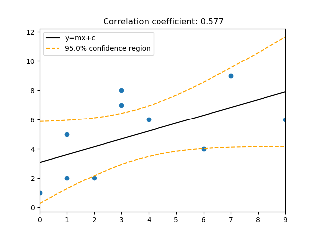
visualisation.plot_regress(x, y, best_fit=True, CI_region=True, CI_slope=False, alpha=0.05, num_plot=111, title='', xlabel='', ylabel='')¶ Produces an x and y scatter plot and calculates the correlation coefficient, as a default it will also plot the line of best fit (using linear regression), and the 95% confidence region.
Parameters: - x (numpy array of dimension 1) –
- y (dependant variable, numpy array of dimension 1) –
- best_fit (True or False depending on whether a line of best fit is) – required, default is set to True.
- CI_region (True or False depending on whether plotting the confidence) – region is required, default is set to True.
- CI_slope (True or False depending on whether the CI slope lines) – are required, default is set to False.
- alpha (required confidence interval (e.g. 0.05 for 95%) Default is 0.05.) –
- num_plot (polot/subplot position, default is 111.) –
- title (title of plot.) –
- xlabel (x axis label.) –
- ylabel (y axis label.) –
Returns: - A scatter plot of x and y, can be visualised using
- plt.show() or saved using plt.savefig()
-
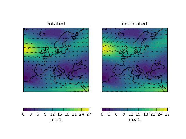
visualisation.vector_plot(u_cube, v_cube, unrotate=False, npts=30, num_plot=111, title='')¶ A plotting function to produce a quick wind vector plot. Output is a plot with windspeed contours and wind vectors. Optionally the u and v components can be unrotated.
Note: If you are unsure whether your winds need to be unrotated you can use http://www-nwp/umdoc/pages/stashtech.html and navigate to the relevant UM version and stash code:
- Rotate=0 means data is relative to the model grid and DOES need to be unrotated.
- Rotate=1 means data is relative to the lat-lon grid and DOES NOT need unrotating.
Parameters: - u_cube (iris 2D cube of u wind component) –
- v_cube (iris 2D cube of v wind component) –
- unrotate (if set to True will unrotate wind vectors, default is False.) –
- npts (integer, plot can look crowded, so plot vector arrow every npts (1=every point, 50=every 50th point), defaults to 30.) –
- num_plot (if subplots required the plot number e.g. 121 can be specified here. Defaults to 111.) –
- title (plot title, must be a string, defaults to blank.) –
utils module
Created on March, 2020 Authors: Chris Kent, Grace Redmond, Saeed Sadri, Hamish Steptoe
-
utils.UMFileList(runid, startd, endd, freq)¶ Give a (thoretical) list of UM date format files between 2 dates. Assuming no missing dates.
Parameters: - runid (model runid) –
- startd (start date(date)) –
- endd (end date(date)) –
- freq –
- frequency of data according to PRECIS technical manual (Specifies) –
- D1 (table) –
- http (//www.metoffice.gov.uk/binaries/content/assets/mohippo/pdf/4/m/tech_man_v2.pdf#page=118) –
- only supports (Currently) –
- pa (Timeseries of daily data spanning 1 month (beginning 0z on the 1st day)) –
- pj (Timeseries of hourly data spanning 1 day (0z - 24z)) –
- pm (Monthly average data for 1 month) –
- currently supported (Not) –
Returns: filelist
Return type: list of strings giving the filenames
Notes
See below for examples
>>> runid = 'akwss'
>>> startd = datetime(1980, 9, 1)
>>> endd = datetime(1980, 9, 3)
>>> freq = 'pa'
>>> print (UMFileList(runid, startd, endd, freq)) # doctest: +NORMALIZE_WHITESPACE
['akwssa.pai0910.pp', 'akwssa.pai0920.pp', 'akwssa.pai0930.pp']
>>> startd = datetime(1980, 9, 1)
>>> endd = datetime(1980, 12, 31)
>>> freq = 'pm'
>>> print (UMFileList(runid, startd, endd, freq)) # doctest: +NORMALIZE_WHITESPACE
['akwssa.pmi0sep.pp', 'akwssa.pmi0oct.pp',
 'akwssa.pmi0nov.pp', 'akwssa.pmi0dec.pp']
-
utils.common_timeperiod(cube1, cube2)¶ Takes in two cubes and finds the common time period between them. This period is then extracted from both cubes. Cubes with common time period are returned, along with strings of the start end end times of the common time period (format DD/MM/YYYY).
Parameters: - cube1 (cube that must have a coord called time.) –
- cube2 (cube that must have a coord called time.) –
Returns: - start_date_str (string of start date for the common period.)
- end_date_str (string of end date for the common period.)
- cube1_common (cube1 with the common time period between cube1 and cube2 extracted.)
- cube2_common (cube2 with the common time period between cube1 and cube2 extracted.)
Notes
The input cubes must have a coordinate called ‘time’ which must have bounds.
An example:
>>> file1 = os.path.join(config.DATA_DIR, 'daily.19990801_19990823.pp')
>>> file2 = os.path.join(config.DATA_DIR, 'daily.19990808_19990830.pp')
>>> cube1=iris.load_cube(file1)
>>> cube2=iris.load_cube(file2)
>>> st, et, c1, c2 = common_timeperiod(cube1, cube2)
Common time period:
('8/8/1999', '23/8/1999')
>>> print(c1.coord('time')[0])
DimCoord([1999-08-08 12:00:00], bounds=[[1999-08-08 00:00:00, 1999-08-09 00:00:00]], standard_name='time', calendar='360_day')
>>> print(c2.coord('time')[0])
DimCoord([1999-08-08 12:00:00], bounds=[[1999-08-08 00:00:00, 1999-08-09 00:00:00]], standard_name='time', calendar='360_day')
>>> print(c1.coord('time')[-1])
DimCoord([1999-08-22 12:00:00], bounds=[[1999-08-22 00:00:00, 1999-08-23 00:00:00]], standard_name='time', calendar='360_day')
>>> print(c2.coord('time')[-1])
DimCoord([1999-08-22 12:00:00], bounds=[[1999-08-22 00:00:00, 1999-08-23 00:00:00]], standard_name='time', calendar='360_day')
-
utils.compare_coords(c1, c2)¶ Compare two iris coordinates - checks names, shape, point values, bounds and coordinate system.
Parameters: - c1 (iris coordinate from a cube) –
- c2 (iris coordinate from a cube) –
Notes
An example:
>>> file1 = os.path.join(config.DATA_DIR, 'gcm_monthly.pp')
>>> file2 = os.path.join(config.DATA_DIR, 'FGOALS-g2_ua@925_nov.nc')
>>> cube1 = iris.load_cube(file1, 'air_temperature')
>>> cube2 = iris.load_cube(file2)
>>>
>>> compare_coords(cube1.coord('latitude'), cube2.coord('latitude'))
long_name values differ: None and latitude
var_name values differ: None and lat
Point dtypes differ: float32 and float64
One has bounds, the other doesn't
-
utils.compare_cubes(cube1, cube2)¶ Compares two cubes for names, data, coordinates. Does not yet include attributes Results are printed to the screen
Parameters: - cube1 (iris cube) –
- cube2 (iris cube) –
Notes
An example:
>>> file1 = os.path.join(config.DATA_DIR, 'gcm_monthly.pp')
>>> file2 = os.path.join(config.DATA_DIR, 'FGOALS-g2_ua@925_nov.nc')
>>> cube1 = iris.load_cube(file1, 'x_wind')
>>> cube2 = iris.load_cube(file2)
>>> compare_cubes(cube1, cube2) # doctest: +NORMALIZE_WHITESPACE
~~~~~ Cube name and data checks ~~~~~
long_name values differ: None and Eastward Wind
standard_name values differ: x_wind and eastward_wind
var_name values differ: None and ua
Cube dimensions differ: 2 and 3
Data dtypes differ: float32 and float64
Data types differ: <class 'numpy.ndarray'> and <class 'numpy.ma.core.MaskedArray'>
~~~~~ Coordinate checks ~~~~~
WARNING - Dimensions coords differ on the following coord(s): ['time']
Checking matching dim coords
-- latitude vs latitude --
long_name values differ: None and latitude
var_name values differ: None and lat
Shapes do not match: (144,) and (145,)
Point values are different
Point dtypes differ: float32 and float64
One has bounds, the other doesn't
-- longitude vs longitude --
long_name values differ: None and longitude
var_name values differ: None and lon
Point values are different
Point dtypes differ: float32 and float64
One has bounds, the other doesn't
WARNING - Dimensions coords differ on the following coord(s): ['air_pressure', 'forecast_period', 'forecast_reference_time', 'height', 'month_number', 'time', 'year']
Cubes have no matching aux coords
-
utils.convertFromUMStamp(datestamp, fmt)¶ Convert UM date stamp to normal python date.
Parameters: - datestamp (UM datestamp) –
- fmt (either 'YYMMM' or 'YYMDH') –
Returns: dt
Return type: datetime object of the input datestamp
Notes
Does not support 3 monthly seasons e.g. JJA as described in the Precis technical manual, page 119.
>>> print (convertFromUMStamp('k5bu0', 'YYMDH'))
2005-11-30 00:00:00
-
utils.convertToUMStamp(dt, fmt)¶ Convert python datetime object or netcdf datetime object into UM date stamp. http://www.metoffice.gov.uk/binaries/content/assets/mohippo/pdf/4/m/tech_man_v2.pdf#page=119
Parameters: - dt (Python datetime object to convert) –
- fmt (either 'YYMMM' or 'YYMDH'. Will not convert seasonal (e.g. JJA)) –
Returns: UMstr
Return type: string with UMdatestamp
Notes
See below for examples
>>> dt = datetime(1981, 11, 2)
>>> print (dt, convertToUMStamp(dt, 'YYMMM'))
1981-11-02 00:00:00 i1nov
>>> print (dt, convertToUMStamp(dt, 'YYMDH'))
1981-11-02 00:00:00 i1b20
>>> dt = cdatetime(1981, 2, 30)
>>> print (dt, convertToUMStamp(dt, 'YYMMM'))
1981-02-30 00:00:00 i1feb
>>> print (dt, convertToUMStamp(dt, 'YYMDH'))
1981-02-30 00:00:00 i12u0
-
utils.date_chunks(startdate, enddate, yearchunk, indatefmt='%Y/%m/%d', outdatefmt='%Y/%m/%d')¶ Make date chunks from min and max date range. Make contiguous pairs of date intervals to aid chunking of MASS retrievals. Where the date interval is not a multiple of yearchunk, intervals of less than yearchunk may be returned.
Parameters: - (string) (enddate) –
- (string) –
- (int) (yearchunk) –
- (string, optional) (outdatefmt) –
- (string, optional) –
Returns: list
Return type: List of strings of date intervals
Notes
This function is only compatible with python 3.
Raises: ValueError– If enddate (ie. max date) is less than or equal to startdate (ie. min date)Excpetion– If yearchunk is not an integerException– If not using python 3
Examples
>>> date_chunks('1851/1/1', '1899/12/31', 25)
[('1851/01/01', '1875/12/26'), ('1875/12/26', '1899/12/31')]
>>> date_chunks('1890/1/1', '1942/12/31', 25)
[('1890/01/01', '1914/12/27'), ('1914/12/27', '1939/12/21'), ('1939/12/21', '1942/12/31')]
-
utils.get_date_range(cube)¶ Takes a cube and calculates the time period spanned by the cube. It returns a string of the start and end date, and an iris constraint that spans the time period of the cube.
Parameters: cube (cube which must include a dimension coordinate called 'time') – Returns: - start_date_str (string of the first time in the cube as a dd/mm/yyyy date)
- end_date_str (string of the last time in the cube as a dd/mm/yyyy date)
- date_range (iris constraint that spans the range between the first and last date)
Notes
See below for an example, this is from a CMIP5 abrupt4xC02 run:
>>> file = os.path.join(config.DATA_DIR, 'FGOALS-g2_ua@925_nov.nc')
>>> cube = iris.load_cube(file)
>>> start_str, end_str, dr_constraint = get_date_range(cube)
0490-11-01 00:00:00
0747-12-01 00:00:00
>>> print(start_str)
1/11/490
>>> print(end_str)
1/12/747
-
utils.precisD2(c)¶ Convert characters according to PRECIS table D2 http://www.metoffice.gov.uk/binaries/content/assets/mohippo/pdf/4/m/tech_man_v2.pdf#page=119
Parameters: - c (character or number to convert) –
- a character to convert from left to right in the table (Supply) –
- an int to convert from right to left in the table (Supply) –
Returns: conv
Return type: converted value: int if input is string, string if input is int
Notes
See below for examples
>>> print (precisD2('1'))
1
>>> print (precisD2('c'))
12
>>> print (precisD2('s'))
28
Also does the reverse conversions: >>> print (precisD2(1)) 1 >>> print (precisD2(12)) c >>> print (precisD2(28)) s
-
utils.precisYY(y)¶ Convert year (int) into 2 character UM year
Parameters: y (int) – Returns: YY Return type: string 2 letter UM year character Notes
See below for an example
>>> print (precisYY(1973))
h3
-
utils.sort_cube(cube, coord)¶ Function to sort a cube by a coordinate. Taken from http://nbviewer.jupyter.org/gist/pelson/9763057
Parameters: - cube (Iris cube to sort) –
- coord (coord to sort by (string)) –
Returns: cube
Return type: a new cube sorted by the coord
Notes
See below for examples
>>> cube = iris.cube.Cube([0, 1, 2, 3])
>>> cube.add_aux_coord(iris.coords.AuxCoord([2, 1, 0, 3], long_name='test'), 0)
>>> print(cube.data)
[0 1 2 3]
>>> cube = sort_cube(cube, 'test')
>>> print(cube.data)
[2 1 0 3]
>>> print(cube.coord('test'))
AuxCoord(array([0, 1, 2, 3]), standard_name=None, units=Unit('1'), long_name='test')
-
utils.umstash_2_pystash(stash)¶ Function to take um style stash codes e.g. 24, 05216 and convert them into ‘python’ stash codes e.g.m01s00i024, m01s05i216
Parameters: stash (a tuple, list or string of stash codes) – Returns: stash_list Return type: a list of python stash codes Notes
Some basic examples:
>>> sc = '24'
>>> umstash_2_pystash(sc)
['m01s00i024']
>>> sc = '24','16222','3236'
>>> umstash_2_pystash(sc)
['m01s00i024', 'm01s16i222', 'm01s03i236']
>>> sc = ['1','15201']
>>> umstash_2_pystash(sc)
['m01s00i001', 'm01s15i201']
Now test that it fails when appropriate:
>>> sc = '-24'
>>> umstash_2_pystash(sc) # doctest: +ELLIPSIS
Traceback (most recent call last):
...
AttributeError: stash item -24 contains non-numerical characters. Numbers only
>>> sc = '1234567'
>>> umstash_2_pystash(sc) # doctest: +ELLIPSIS
Traceback (most recent call last):
...
IndexError: stash item is 1234567. Stash items must be no longer than 5 characters
>>> sc = 'aaa'
>>> umstash_2_pystash(sc) # doctest: +ELLIPSIS
Traceback (most recent call last):
...
AttributeError: stash item aaa contains non-numerical characters. Numbers only
>>> sc = '24a'
>>> umstash_2_pystash(sc) # doctest: +ELLIPSIS
Traceback (most recent call last):
...
AttributeError: stash item 24a contains non-numerical characters. Numbers only
>>> sc = 24, 25
>>> umstash_2_pystash(sc) # doctest: +ELLIPSIS
Traceback (most recent call last):
...
TypeError: 24 must be a string